Problem formulation

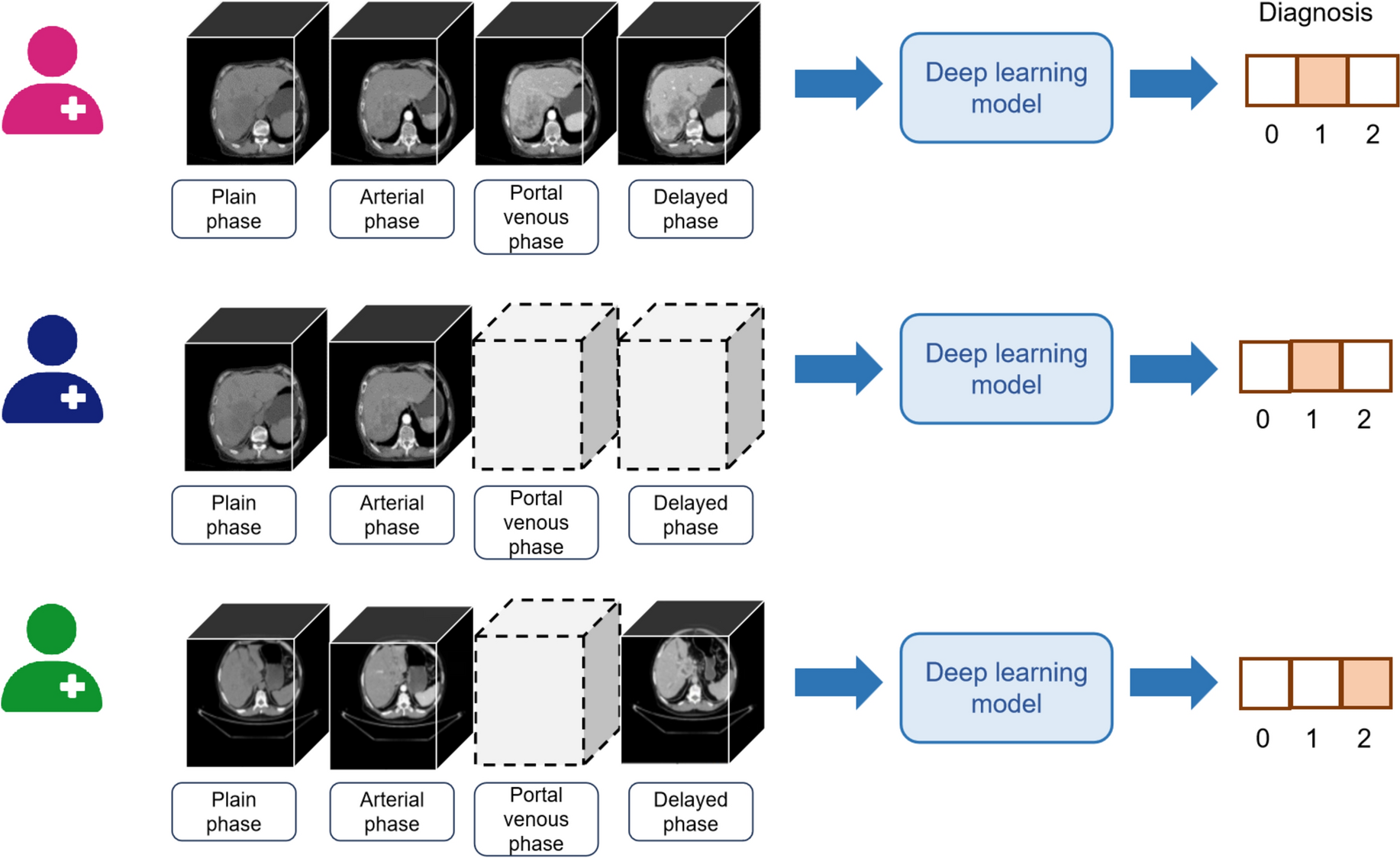
For a given patient \(\:i\), the diagnostic prediction is based on a combination of images from the four available phases: plain phase \(\:\left(}_\right)\), arterial phase \(\:\left(}_\right)\), venous phase \(\:\left(}_\right)\), and delayed phase \(\:\left(}_\right)\). Since contrast-enhanced CT (CECT) images from the plain phase are always present during the diagnosis of primary liver cancers for comprehensive assessment of liver lesions, the input for diagnostic prediction must include the plain phase and at least one additional phase image. The diagnostic prediction outcome, \(\:_\), can take values from the set \(\:\,2\}\), representing normal individuals, hepatocellular carcinoma, and intrahepatic cholangiocarcinoma, respectively. For a detailed illustration of the diagnostic process and phase combinations, see Fig. 1.

Fig. 1

Diagnosis prediction of patients based on variable multi-phase CECT. Dashed boxes indicate the absence of CECT images for that phase of the patient. 0, 1, and 2 represent individuals with normal conditions, HCC, and ICC, respectively

Model structure

As illustrated in Fig. 2, our proposed H-LSTM network comprises an image feature extractor shared by all phases of 3D CECT images, four phase-specific intra-phase BiLSTM networks, one phase index embedding network, an inter-phase BiLSTM network, and an output layer. Each phase’s 3D CECT is initially processed by the shared feature extractor for feature extraction. Subsequently, the extracted features of different tiers within each phase are integrated using the phase-specific BiLSTM. These integrated features are then concatenated with the output from the phase index embedding network, followed by the application of the inter-phase BiLSTM to aggregate features across different phases. Finally, the aggregated features are fed into the output layer for classification and prediction.

Fig. 2

Model Architecture Diagram. The figure illustrates the diagnostic classification process of the model for an individual with CECT images in all four phases. CN, HCC, and ICC respectively denote normal, Hepatocellular Carcinoma, and Intrahepatic Cholangiocarcinoma

Image feature extractor

The purpose of the image feature extractor is to extract features from CECT images across different phases. We have selected ResNet (Sarwinda et al. 2021), VGGNet (Simonyan 2014), DenseNet (Huang 2017), InceptronNet (Szegedy 2015) and EfficientNet (Tan 2019) as candidate networks. The rationale behind choosing these well-known networks is the availability of a substantial number of pre-trained model parameters. Through transfer learning (Gao et al. 9,33,34,; Aslan et al. 2021), we can finetune these parameters to build a local model that is specific to our task on a limited dataset. Leveraging pre-trained model parameters is advantageous because these models have already learned to extract general image features, which can accelerate the convergence of our model and enhance its performance. Within each phase, we map the images\(\:}_\) to a vector \(\:_\in\:\)\(^}}\) using the feature extractor, as depicted in Eq. (1). \(\:f\) represents the feature extractor, and \(\:\theta\:\) denotes its parameters.

$$\:\begin_=f\left(}_;\theta\:\right)\end$$

(1)

Internal LSTM

Next, we address the aggregation of CECT images with varying numbers of layers using a BiLSTM. The forward computation process of the BiLSTM is detailed in Eqs. (2, 3). This sequential architecture aids in capturing the structural information of the liver stored within the CECT data.

LSTM-Forward:

$$\begin f_k^f = sigmoid\left( + U_f^fh_^f + b_f^f} \right), \hfill \\ i_k^f = sigmoid\left( + U_f^ih_^f + b_f^i} \right) \hfill \\ \tilde c_k^f = \tanh \left( + U_f^gh_^f + b_f^g} \right), \hfill \\ c_k^f = f_k^f \circ c_^f + i_k^f \circ \tilde c_k^f, \hfill \\ o_k^f = sigmoid\left( + U_f^oh_^f + b_f^o} \right), \hfill \\ h_k^f = o_k^f \circ \tanh \left( \right) \hfill \\ \end$$

(2)

LSTM-Backward:

$$\begin f_k^b = sigmoid\left( + U_f^fh_^f + b_b^f} \right), \hfill \\ i_k^b = sigmoid\left( + U_f^ih_^f + b_b^i} \right) \hfill \\ \tilde c_k^b = \tanh \left( + U_f^gh_^f + b_b^g} \right), \hfill \\ c_k^b = f_k^b \circ c_^b + i_k^b \circ \tilde c_k^b, \hfill \\ o_k^b = sigmoid\left( + U_f^oh_^f + b_b^o} \right), \hfill \\ h_k^b = o_k^b \circ \tanh \left( \right) \hfill \\ \end$$

(3)

The superscript \(\:b\) indicates backward propagation, and \(\:f\) indicates forward propagation. The equations above describe a BiLSTM, where there are two directions of hidden state propagation, each with its own set of weight matrices and biases. The input sequence is denoted as \(\:_\), and the hidden state \(h_\) incorporates information from both forward and backward propagation. The hidden states for forward and backward propagation are denoted as \(h_k^f\) and \(h_k^b\), respectively, and they are computed based on the input from both directions as well as the hidden state from the previous time step.

We aggregated these vectors using a phase-specific BiLSTM to obtain \(\:_\), allowing the LSTM to capture spatial relationships between different layers in an ordered manner. This BiLSTM is also referred to as an internal LSTM. \(\:_\) represents the feature representation of the CECT images for the \(\:j\)-th phase, encapsulating the semantic information for that phase. See Eq. (4) for details.

$$\begin h_}}^f = LST\left( },}, \ldots ,}}}} \right],h_o^f} \right), \hfill \\ h_}}^b = LST\left( },}, \ldots ,}}}} \right],h_o^b} \right) \hfill \\ \end$$

(4)

Therefore, \(\:_\) is obtained by concatenating \(h_k^f\) and \(h_k^b\), as shown in Eq. (5),

$$} = \left[ }}^f;h_}}^b} \right]$$

(5)

where \(\:_\) represents the number of layers of a CECT image.

Phase index embedding

Next, to establish the correspondence between images and phases, we encoded the index \(\:j\) of each phase as a one-hot vector and then mapped it to a vector \(\:_\in\:^}}\) using an embedding matrix \(\:^\in\:^}}\) (Eq. (6). We concatenated \(\:_\) and \(\:_\) to obtain \(\:_=[_;_]\). This augmentation with \(\:_\) incorporates information about the phase, in addition to the features in \(h_\).

$$\:\begin_=onehot\left(j\right)\cdot\:^\end$$

(6)

External LSTM

Subsequently, we input \(\:[_\mid\:j\in\:\,\text\left\}\right]\) into a BiLSTM to aggregate semantic features from different phases, facilitating the learning of associations between images across various phases. We refer to this BiLSTM as the external LSTM. Apart from the input, the forward computation process of the external LSTM is identical to that of the internal LSTMs in each phase, as illustrated in Eq. (7).

$$\begin h_i^f = LST\left( }} \right],h_o^f} \right), \hfill \\ h_i^b = LST\left( }} \right],h_o^b} \right) \hfill \\ \end$$

(7)

Output layer

Finally, we established a prediction layer, which comprises a single-layer fully connected neural network, to generate a vector of length 3 as the output. We applied the softmax activation function to this output, allowing us to make predictions for the diagnostic outcomes (normal, HCC, or ICC) for patient \(\:i\), as illustrated in Eq. (8).

$$ = s}\left( \left[ \right] + } \right)$$

(8)

Loss function

We constructed the cross-entropy loss function based on the real diagnosis of patients, denoted as \(\:_\), and the predicted values, denoted as \(\:}_\), as shown in Eq. (9).

$$\:\begin\mathcal L=-\frac\sum\:_^\:\sum\:_^\:_\cdot\:log\left(}_\right)+\lambda\:|\left|\right|_^\end$$

(9)

In this context, \(\:\) represents all the model parameters to be learned, and \(\:\lambda\:\) is the coefficient for L2 regularization.

Experimental configurationDataset

The dataset utilized in this research was gathered from the Chongqing Yubei District People’s Hospital, Chongqing Wanzhou Three Gorges Central Hospital, and the Radiology Departments of Southwest Hospital. It encompasses a total of 276 participants, segmented into three distinct groups. The normal group consists of 83 individuals who underwent routine physical examination CECT scans, revealing no liver or bile duct abnormalities. The diseased group is composed of 193 individuals, including 94 cases of Hepatocellular Carcinoma and 99 cases of Intrahepatic Cholangiocarcinoma, all confirmed by pathological examination to be primary liver cancer. This dataset offers two subtypes of primary liver cancer cases, providing a robust basis for a comprehensive analysis and evaluation of the proposed methods. For a detailed account of the patient selection process and the inclusion and exclusion criteria, refer to Fig.A1.

Data preprocessing

Liver cancer CECT scans typically comprise four phases: plain, arterial, venous, and delayed. The CECT images for each phase are three-dimensional with dimensions \(\:_\times\:512\times\:512\), where \(\:_\) varies. Here, \(\:i\) denotes the patient’s index, and \(\:j\) indicates the phase. We rescale each phase to \(\:_\times\:224\times\:224\) using cubic interpolation. The purpose of rescaling to \(\:224\times\:224\) is to facilitate the use of most pre-trained mature networks for transfer learning, which is particularly crucial for small-sample medical data. Moreover, to adapt the data for direct modeling with 3D network structures like 3D-ResNet, we uniformly rescale the images to \(\:60\times\:224\times\:224\), where 60 represents the number of layers. We then concatenate the CECT images from all four phases along the channel dimension, resulting in a final dimension of \(\:60\times\:224\times\:224\times\:4\).

We constructed scenarios of incomplete phase data based on the complete phase datasets. Specifically, in real clinical settings, every patient must have a plain phase CECT scan. Thus, when creating the incomplete phase dataset, we assumed that each patient would have at least the plain phase, ensuring that any given patient \(\:i\) would have at least two CECT phases, one of which is the plain phase. Let \(\:_\) represent the total number of CECT phases available for patient \(\:i\). During model training, we randomly removed 0–2 phases, excluding the plain phase. After removal, each patient \(\:i\) would have 2–4 CECT phases, simulating a scenario with missing phases. This augmentation strategy ensures that each training sample includes at least two CECT phases, enabling us to model more complex scenarios with missing phase data and enhance the model’s generalization ability.

Model comparison

For the H-LSTM network, we employed various feature extractors to assess their impact on performance. Additionally, we experimented with replacing the BiLSTM structure with a Transformer architecture, which we refer to as the Hierarchical Transformer (H-Transformer). Furthermore, we utilized a 3D-ResNet to directly classify and predict across multiple phases of images for individual patients.

Implementation details

We employed a stratified randomization approach to partition the dataset, ensuring that the training, testing, and validation sets maintained class balance within the hepatocellular carcinoma (HCC), intrahepatic cholangiocarcinoma (ICC), and normal populations. Specifically, the dataset was divided into training, testing, and validation sets in a 7:2:1 ratio, as shown in Table 1. This approach was essential to maintain class balance across the various datasets.

Table 1 Composition of patients from different categories in various datasets

For the feature extractor, we utilized pre-trained models from the ImageNet dataset, obtained through the torchvision package. The rationale for selecting these models (e.g., ResNet, DenseNet) was their proven performance in medical imaging tasks and the availability of well-established, transferable parameters. We then fine-tuned these parameters in an end-to-end manner while training the H-LSTM model. The Adam optimizer was used due to its efficiency in handling sparse gradients and its ability to adjust learning rates dynamically. Detailed hyperparameter settings are presented in Table 2. The training set was employed for model parameter training, while the validation set was used for hyperparameter tuning and implementing an ‘early stopping’ strategy. Specifically, we stipulated that training would halt if there was no improvement in performance on the validation set for two consecutive epochs. The model that achieved the highest AUC on the validation set was selected as the final model and subsequently evaluated on the test set.

Table 2 List of hyperparameters for model constructionEvaluation metrics

To assess the performance of our classification model, we employed the following metrics: Accuracy, Recall (Sensitivity), Precision, F1 Score, Area Under the Receiver Operating Characteristic Curve (AUROC), and Area Under the Precision-Recall Curve (AUPRC). For multi-class classification problems, we employed the “macro” averaging method to calculate each metric across all classes. This approach treats all classes with equal importance. Bootstrap resampling was utilized to estimate confidence intervals for each metric, providing a measure of statistical reliability. All results were reported based on the test dataset.