
記住我

Approaches for quantitative bias analysis have been well described in the epidemiologic literature, yet uptake of such methods remains low.1 There are textbooks on the topic,2 including user-friendly spreadsheets, add-on software packages for Stata3 and R, and SAS macros.4 In 2014, Lash and colleagues1 suggested that a key barrier to implementation is that researchers may lack training in quantitative bias analysis approaches. However, nearly 10 years later, there is still a tendency for authors to provide qualitative descriptions of potential bias rather than a quantitative assessment of the magnitude and direction of bias. Improving the uptake of quantitative bias analysis requires both increased training opportunities and accessible tools to facilitate the implementation of such approaches.
In this manuscript, we describe the use of Apisensr, a web-based application designed for quantitative bias analysis. This tool enables epidemiologists and other health science researchers to incorporate quantitative bias analysis into their work. A key benefit of Apisensr is that it does not require any statistical software or programming expertise; thus, it is designed for researchers who possess foundational knowledge about bias but need assistance with the implementation of bias analyses. Apisensr is freely available online at https://dhaine.shinyapps.io/apisensr/. It is an easy-to-use web-based Shiny app that implements the code available in the R package episensr, or, equivalently, Stata’s episens package. Additional information about episensr including conceptual descriptions of quantitative bias analysis can be found on GitHub at https://dhaine.github.io/episensr/articles/episensr.html. Apisensr can be used for quantitative bias analysis for selection bias, unmeasured confounding, and misclassification, for simple bias analysis, or probabilistic bias analysis. It can be used for differential and nondifferential misclassification of exposure or outcome. There are options to conduct simple bias analysis using data (i.e., entering a 2 × 2 table) or based on observed relationships between variables. For probabilistic analyses, there are options to set the starting seed and vary the number of simulations to be run. It is very easy to explore the impact of varying bias parameter values on study results by using a slider bar to increase or decrease the amount of bias present. It is programmed to request the relevant bias parameter values required for a specific type of bias analysis, such as sensitivity and specificity values for analysis of misclassification or sampling fractions for selection bias. Results can be output as risk ratios, odds ratios, or risk differences, depending on user preferences. Further, for probabilistic analyses, the user has the option to select whether they want the simulation interval around the effect estimates adjusted for just systematic error or both random and systematic errors. The output also includes a plot of bias-adjusted effect estimates from each simulation run. Finally, Apisensr comes populated with sample data, meaning that it can be easily incorporated into class lectures for teaching purposes so students can see the quantitative impact of increasing or decreasing bias on an effect estimate.
In this manuscript, we demonstrate the use of Apisensr to adjust for misclassification bias. First, we quantify misclassification of obesity status due to the use of self-reported body mass index (BMI) (kg/m2) and then examine the effect of misclassification on the association between obesity and diabetes.
APPLICATION: MISCLASSIFICATION OF OBESITY STATUS DUE TO THE USE OF SELF-REPORTED BMIMeasurement bias is a form of systematic error that occurs when study variables are incorrectly measured. Mismeasurement of exposure, outcomes, or covariates can produce bias in effect estimates.2,5–12 This type of bias is often called misclassification when referring to incorrect categorization of binary or categorical variables.13–15 A frequently discussed type of misclassification bias is related to the use of self-reported variables.16 While self-report of exposure status has several advantages, it comes at a cost of potentially reduced accuracy relative to the true measured exposure. Self-reported BMI is often used in epidemiologic analyses, given the challenges associated with obtaining measured body weight and height in large epidemiologic cohorts. The accuracy of self-reported BMI may be affected by several factors including poor recall, social desirability, and whether the participant believes their data will be independently verified (i.e., through medical records) or objectively measured at a subsequent time point.17 Using self-reported BMI to define obesity status may result in misclassification.18–20 Prior evidence also demonstrates that the degree of accuracy in reporting may differ for individuals from different demographic groups, such as age, sex, and race–ethnicity.16,21
Frequently, a cut point of BMI ≥30 kg/m2 is used to define obesity status, in line with numerous clinical and public health guidelines (e.g., World Health Organization,22 American Heart Association,23 and American Diabetes Association24). The consequences of inaccurate self-reported BMI may be compounded when examining a dichotomous variable, such as obesity status.25 Inaccuracy of a continuous variable may lead to individuals being incorrectly classified into exposure categories.6,25 As demonstrated by Flegal et al.,6 the probability of misclassification is likely to be higher for individuals with BMI values close to the categorical cut point chosen. For individuals with true BMI values close to the cut point of 30 kg/m2, only a small degree of error in self-reported height or weight could result in them being misclassified as obese when truly nonobese or vice versa. Even if the measurement error in the underlying continuous variable is nondifferential, or unrelated to outcome status, the misclassification bias introduced by categorizing that variable may be either nondifferential or differential.6 When there is a causal relationship between the exposure and outcome, individuals with BMI values just below the cut point of 30 kg/m2 are more likely to have the outcome than individuals with lower BMI values (i.e., further below 30 kg/m2). If the probability of outcome differs within a category of the exposure, differential misclassification may be introduced, even if the mismeasurement of the underlying continuous variable was nondifferential.6
METHODS Study PopulationWe used publicly available data from the National Health and Nutrition Examination Survey (NHANES), a series of nationally representative cross-sectional surveys of civilians in the United States.26,27 For the purpose of estimating the bias parameter values required for the quantitative bias analysis, we used a sample of 41,243 adults 18–79 years who participated in NHANES 1999–2012 waves. Participants completed an in-home interview and a physical examination at a mobile examination center. The in-home interview includes health interviews by trained examiners and questionnaires.28 The physical examination includes clinical laboratory tests, biospecimen collection, interviews via computer-assisted interviewing system, and standardized measurements.28 According to NHANES procedures manuals, the average time between in-home interview and physical examination is 2 weeks.28 To demonstrate the use of Apisensr and emulate a scenario in which researchers want to apply estimated bias parameter values to an external dataset, we used data on adults 18–79 years who participated in NHANES between 2017 and 2020 (N = 15,560). All participants provided written informed consent and the NHANES study protocol was approved by the National Center for Health Statistics Institutional Review Board. All data are available for download at: https://www.cdc.gov/nchs/nhanes/index.htm.
Measures Self-reported and Measured BMISelf-reported height and weight estimates were ascertained during a household interview. Participants were asked to recall their current height and weight via questionnaire: “How tall are you without shoes?” “How much do you weigh without clothes or shoes?”27 Self-reported height was reported in inches and weight in pounds that were later converted to meters (m) and kilograms (kg), respectively. Measured height and weight estimates were collected at the physical examination mobile examination centers by trained health professionals.26 Weight was measured in kilograms while participants were dressed in a disposable hospital examination gown without shoes and standing height was measured using a stadiometer platform in centimeters.27 Participants provided written informed consent and were given the opportunity to review all measures collected via home visit and mobile examination before participation. This data collection structure could have influenced the validity of self-reported height and weight because participants were aware these measures would also be recorded during the subsequent planned visit to the examination center. Self-reported and measured height and weight were used to calculate BMI (kg/m2). Obesity was defined as BMI ≥30 kg/m2.
CovariatesFor this analysis, we examined differences in self-reported and measured BMI according to race–ethnicity (Mexican or Hispanic American, non-Hispanic (NH) White, NH Black, and other/multirace groups), sex (male, female), and age (18–40, 40–59, 60–79 years). NHANES records sex as a self-reported binary variable (i.e., male and female) so this is how we used the variable in our analyses. Age was assessed at the time of the household interview screening and was reported in years. After 2007, NHANES coded participants 80 or older as 80 years of age; but, in the 1999–2006 waves, individuals 85 years and older were top-coded as 85.29 Due to these discrepancies between waves, we restricted our analytic sample to adults less than 80 years of age.
Statistical AnalysisDescriptive statistics were calculated for the total sample from NHANES 1999–2012 (N = 41,243). Survey weights were used to account for the complex sampling design of the NHANES survey.28 Means and corresponding 95% confidence intervals (CIs) were calculated for both self-reported and measured height, weight, and BMI by sex, age category, and race. We calculated the difference between self-reported and measured BMI as self-reported minus measured BMI.
We then estimated bias parameter values comparing obesity (BMI ≥30 kg/m2) defined by self-reported BMI with obesity defined by measured BMI. As an extension, we also describe an approach for estimating bias parameter values for BMI categories comparing self-reported BMI and measured BMI. We applied the bias parameter values for obesity to adjust for exposure misclassification using Apisensr.
Estimating Bias Parameter ValuesFor an analysis of exposure misclassification, there are four relevant bias parameters: sensitivity, specificity, positive predictive value (PPV), and negative predictive value (NPV).2 These bias parameter values are calculated by comparing the gold-standard measurement, obesity defined by measured BMI, with the index measurement, self-reported BMI. Sensitivity is the ability of a test to correctly identify individuals who are positive, and specificity is the ability of a test to correctly identify individuals who are negative. In the context of comparing self-reported and measured obesity, sensitivity refers to the proportion of individuals who are correctly identified as having obesity according to their self-reported BMI compared to being identified as having obesity by measured BMI. Specificity refers to the proportion of individuals who were correctly identified as not having obesity according to their self-reported BMI compared to measured BMI. PPV is the probability of self-reporting as obese (BMI ≥30 kg/m2) conditional on truly being in that BMI category while NPV is the probability of a not self-reporting obese conditional on an individual truly not being in that category (according to measured BMI). We calculated bias parameter values and corresponding 95% CIs for each combination of age, sex, and race–ethnicity to examine potential differences in the degree of misclassification of obesity status. In this analysis, we assumed misclassification is nondifferential by outcome status. However, as a sensitivity analysis, we also calculated the bias parameters within strata of the outcome (diabetes). Given sample size limitations, we were not able to calculate bias parameter values stratified by age, sex, and race–ethnicity and also outcome status.
Quantitative Bias Analysis Using ApisensrWe used Apisensr to examine potential bias due to the use of self-reported BMI in an analysis of the association between obesity (BMI ≥30 kg/m2) and diabetes. In this analysis, we stratified according to the same age, sex, and race–ethnicity categories described above. The relationship between high BMI and diabetes is well known; having obesity is a strong risk factor for diabetes.30 Based on prior research, we expect a strong positive relationship between high BMI and prevalent diabetes. Our interest here is in examining the magnitude and direction of bias due to exposure misclassification, rather than a novel epidemiologic finding regarding the exposure outcome relationship. In Apisensr, the user enters the crude observed data (i.e., 2 × 2 table of data on obesity and diabetes) and bias parameter values for sensitivity and specificity. We used a probabilistic bias analysis approach to calculate a bias-adjusted prevalence odds ratio. Probabilistic bias analysis requires the user to specify a probability distribution around the sensitivity and specificity values and uses Monte Carlo sampling of bias parameter values from the probability distribution.2 In this example, we chose a triangular distribution with the mode corresponding to the stratum specific sensitivity and specificity. The lower and upper limits of the triangular distribution corresponded to the 95% CIs for the sensitivity and specificity values. Apisensr allows for different specifications for the probability distribution, including uniform, triangular, trapezoidal, log-normal, log-logistic, and beta. We also verified the results from Apisensr with Stata’s episens package.3 For readers interested in replicating our approach using NHANES 2017–2020 data, we report the observed data (cell counts) in Table 5. This crude, stratified data can be entered into Apisensr along with the bias parameters estimated in Table 3 to gain hands-on experience in conducting bias analysis using real-world data.
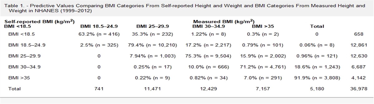
Extension: Estimating Bias Parameter Values for a Categorical VariableIn the main analysis presented in this manuscript, we compared obesity defined by self-reported BMI with obesity defined by measured BMI, focusing on a misclassified dichotomous variable. However, it may also be of interest to some readers to estimate bias parameter values for a misclassified categorical variable. To demonstrate this approach, we created two new variables using data from NHANES 1999–2012: a five-level categorical variable from self-reported BMI and a five-level categorical variable from measured BMI. The BMI categories were (1) BMI <18.5 kg/m2, (2) BMI 18.5–24.9 kg/m2, (3) BMI 25–29.9 kg/m2, (4) BMI 30–34.9 kg/m2, and (5) BMI ≥35 kg/m2. In Table 1, we present a cross-tabulation of self-reported BMI and measured BMI categories. The percentages reported along the diagonal are equivalent to PPVs, calculated as the probability of being in a self-reported BMI category conditional on being in the corresponding measured BMI category. For instance, there were 9504 individuals with measured BMI 25–29.9 kg/m2 of 12,630 individuals who self-reported BMI 25–29.9 kg/m2 (9,504/12,630 = 75.3%) and there were 4761 kg/m2 individuals with measured BMI 30–34.9 kg/m2 of 6687 individuals who self-reported BMI 30–34.9 kg/m2 (4,761/6,687 = 71.2).
Table 1. - Predictive Values Comparing BMI Categories From Self-reported Height and Weight and BMI Categories From Measured Height and Weight in NHANES (1999–2012) Self-reported BMI (kg/m2) Measured BMI (kg/m2) BMI <18.5 BMI 18.5–24.9 BMI 25–29.9 BMI 30–34.9 BMI >35 Total BMI <18.5 63.2% (n = 416) 35.3% (n = 232) 1.22% (n = 8) 0.3% (n = 2) 0 658 BMI 18.5–24.9 2.5% (n = 325) 79.4% (n = 10,210) 17.2% (n = 2,217) 0.79% (n = 101) 0.06% (n = 8) 12,861 BMI 25–29.9 0 7.94% (n = 1,003) 75.3% (n = 9,504) 15.9% (n = 2,002) 0.96% (n = 121) 12,630 BMI 30–34.9 0 0.25% (n = 17) 10.0% (n = 666) 71.2% (n = 4,761) 18.6% (n = 1,243) 6,687 BMI >35 0 0.22% (n = 9) 0.82% (n = 34) 7.0% (n = 291) 91.9% (n = 3,808) 4,142 Total 741 11,471 12,429 7,157 5,180 36,978The percentages presented in the off-diagonal cells have an interpretation similar to a NPV, the proportion of individuals with a given self-reported BMI value that are truly “negative” (i.e., not in that category according to measured BMI). For example, among the 12,630 individuals that self-reported having a BMI 25–29.9 kg/m2, 7.9% had a measured BMI 18.5–24.9 kg/m2, 15.9% had measured BMI 30–34.9 kg/m2, and 0.96% had a measured BMI ≥35 kg/m2. The sum total of the off-diagonal percentages in each row of the table can be taken as the proportion of individuals in the measured BMI categories that are different from the given self-reported BMI value. An important consideration with a self-reported categorical variable is the fact that there is potential for misclassification in two directions, both above and below the true measured category. To correctly reclassify participants, categorical predictive values must be combined with a probabilistic process to account for the potential for misclassification. To do so, draw from a probability distribution (i.e., uniform, normal) for each participant in the dataset and reclassify the participants using the predictive values. Sample Stata code corresponding to the predictive values for misclassification of BMI categories is included in the eAppendix; https://links.lww.com/EDE/C114.
RESULTSDemographic characteristics of NHANES 1999–2012 study participants are presented in Table 2. There were 16,454 individuals who were 18–39 years old, 11,584 who were 40–59 years old, and 10,093 who were 60–69 years old. The sample was 48% male. Overall, mean measured BMI was higher than self-reported BMI (28.3 kg/m2 vs. 27.6 kg/m2 ± 5.9 kg/m2). Self-reported height was slightly larger than measured height and self-reported weight was 0.9 kg smaller than measured weight. Table 3 presents differences between self-reported and measured height, weight, and BMI according to age (18–39, 40–59, and 60–79 years), sex (male, female), and race–ethnicity (Mexican or Hispanic, NH White, NH Black, other/multirace). Both men and women of all ages and race–ethnicity groups overreported their height. In general, the discrepancy between measured and self-reported height was greater for men than women. Men and women in the oldest age group (60–79 years) were more likely to overreport their height compared to younger individuals. Women underreported their weight to a greater degree than men. The discrepancy between self-reported and measured weight was largest for women in the youngest age group (NH White women: −2.72 kg, NH Black women: −2.64 kg, Mexican/Hispanic women: −1.79 kg, other/mixed race: −1.98 kg). The combined result of misreporting height and weight is reflected in BMI measures. BMI in women was 0.9 kg/m2 lower when using self-reported height and weight to calculate BMI compared to 0.5 kg/m2 lower in men. NH White, NH Black, and Hispanic women in the 18–39-year age group had a BMI difference ≥1 kg/m2 (NH White women: −1.12 kg/m2, NH Black women: −1.14, Hispanic women: −1.01 kg/m2).
Table 2. - Demographic and Anthropometric Characteristics of NHANES Study Participants From 1999 to 2012 (N = 41,243) Age at screening, n (%) 18–39 yr 16,454 (43%) 40–59 yr 11,594 (38%) 60–79 yr 10,093 (19%) Sex, n (%) Female 21,337 (52%) Male 19,906 (48%) Race/ethnicity, n (%) Non-Hispanic White 18,903 (70%) Non-Hispanic Black 8,799 (11%) Mexican/Hispanic 11,034 (13%) Other/ Multirace 2,507 (6%) Survey cycle, n (%) NHANES 1999–2000 5,448 (13%) NHANES 2001–2002 5,993 (14%) NHANES 2003–2004 5,620 (14%) NHANES 2005–2006 5,563 (14%) NHANES 2007–2008 6,228 (15%) NHANES 2009–2010 6,527 (15%) NHANES 2011–2012 5,864 (15%) Self-reported height (m); mean ± SD 1.70 ± 0.001 Self-reported weight (kg); mean ± SD 80.1 ± 0.19 Measured height (m); mean ± SD 1.68 ± 0.001 Measured weight (kg); mean ± SD 81.0 ± 0.21 Measured BMI (kg/m2); mean ± SD 28.3 ± 0.07 Self-reported BMI (kg/m2); mean ± SD 27.6 ± 0.06 Proportions and means weighted by NHANES sampling weights 1999–2012 to account for the complex survey design.28SD indicates standard deviation.
Table 4 presents bias parameter values of sensitivity, specificity, PPV, and NPV stratified by age, sex, and race–ethnicity comparing obesity (BMI ≥30 kg/m2) defined by self-reported compared with measured BMI. These are the values that could be applied by other researchers interested in conducting quantitative bias analysis to adjust for the use of self-reported obesity in their own work. Given the dependence of PPV and NPV on prevalence, caution must be exercised if transporting these bias parameter values to other study populations; appropriate use of the sensitivity and specificity values presented would be a better choice. The prevalence of measured obesity, accounting for NHANES sampling weights, is also included in Table 4. In men and women, the prevalence of obesity was highest in non-Black individuals. The prevalence of obesity in NH Black men was 30.8% for those aged 18–39 years, 36.1% for those aged 40–59 years, and 36.3 for those 60-79 years. In NH Black women, prevalences were 48.5% for those aged 18–39 years, 55.1% for those aged 40–59 years, and 57.5% for those aged 60–79 years. Prevalence of obesity was lowest in young, NH White men and women: 25.0% for men and 26.1% for women. There was variation in the bias parameter values across strata, indicating the potential magnitude of misclassification bias differs according to age, sex, and race–ethnicity categories. Sensitivity and specificity measures were generally high across all demographic groups (sensitivity range: 75%–89%; specificity range: 91%–99%). Sensitivity analyses to explore nondifferential misclassification by outcome demonstrate little variation in bias parameter values by diabetes status. For individuals with diabetes, sensitivity was 87% (95% CI = 85, 89), specificity was 95% (95% CI = 93, 97), PPV was 96% (95% CI = 94, 97), and NPV was 84% (81%, 87%). Among individuals without diabetes, sensitivity was 83% (95% CI = 81, 84), specificity was 97% (95% CI = 96, 98), PPV was 94% (95% CI = 93, 95), and NPV was 92% (95% CI = 91, 93). This suggests that misclassification of obesity status may not be differential according to diabetes status.
Table 4. - Prevalence and Bias Parameter Values Comparing Obesity Defined Using Self-reported BMI With Obesity Defined by Measured BMI in NHANES 1999–2012 (N = 41,243) N True Prevalence of Obesity Sensitivity Specificity Positive Predictive Value Negative Predictive Value Men, aged 18–39 yr Non-Hispanic White 2,822 25.0% 83.7% (80.7, 86.4) 98.2% (97.5, 98.7) 93.8% (91.6, 95.5) 94.8% (93.8, 95.7) Non-Hispanic Black 1,684 30.8 % 85.2% (81.7, 88.3) 97.1% (96.0, 98.0) 92.2% (89.3, 94.6) 94.3% (92.8, 95.5) Mexican/Hispanic 2,254 28.7% 79.3% (75.6, 82.6) 94.8% (93.6, 95.9) 84.5% (81.0, 87.5) 92.8% (91.4, 94.0) Men, aged 40–59 yr Non-Hispanic White 2,504 35.7% 84.5% (82.0, 86.8) 96.5% (95.4, 97.3) 92.9% (90.9, 94.6) 91.9% (90.5, 93.2) Non-Hispanic Black 1,191 36.1% 85.8% (82.1, 88.9) 95.3% (93.6, 96.7) 91.3% (88.1, 93.9) 92.1% (90.0, 93.9) Mexican/Hispanic 1,400 33.9% 81.0% (77.1, 84.5) 91.2% (89.1, 93.0) 82.8% (78.9, 86.2) 90.2% (88.0, 92.0) Men, aged 60–79 yr Non-Hispanic White 2,337 36.2% 81.7% (78.9, 84.3) 98.2% (97.4, 98.8) 96.2% (94.5, 97.5) 90.7% (89.2, 92.0) Non-Hispanic Black 1,005 36.3% 82.1% (77.7, 85.9) 94.5% (92.4, 96.1) 89.3% (85.5, 92.5) 90.4% (87.9, 92.5) Mexican/Hispanic 1,108 33.5% 76.6% (71.9, 80.9) 95.2% (93.4, 96.7) 89.2% (85.1, 92.4) 88.8% (86.3, 91.0) Women, aged 18–39 yr Non-Hispanic White 3,201 26.1% 77.3% (74.4, 80.1) 99.2% (98.8, 99.5) 97.3% (95.8, 98.4) 92.3% (91.2, 93.4) Non-Hispanic Black 1,826 48.5% 83.8% (81.0, 86.3) 97.4% (96.2, 98.3) 96.3% (94.6, 97.5) 88.1% (86.1, 90.0) Mexican/Hispanic 2,617 34.6% 75.0% (71.7, 78.1) 97.3% (96.3, 98.0) 92.8% (90.4, 94.7) 89.2% (87.7, 90.7) Women, aged 40–59 yr Non-Hispanic White 2,450 35.7% 87.8% (85.4, 89.8) 98.5% (97.8, 99.1) 97.3% (95.9, 98.3) 93.1% (91.8, 94.3) Non-Hispanic Black 1,304 55.1% 88.8% (86.2, 91.0) 94.3% (92.1, 96.0) 95.0% (93.0, 96.5) 87.3% (84.5, 89.8) Mexican/Hispanic 1,456 45.4% 83.3% (80.1, 86.2) 94.9% (93.0, 96.4) 93.3% (90.9, 95.3) 86.8% (84.3, 89.1) Women, aged 60–79 yr Non-Hispanic White 2,219 37.5% 79.7% (76.7, 82.4) 98.8% (98.0, 99.3) 97.4% (95.9, 98.5) 89.1% (87.4, 90.6) Non-Hispanic Black 990 57.5% 85.8% (82.6, 88.7) 94.5% (91.8, 96.5) 95.3% (93.0, 97.0) 83.6% (80.0, 86.8) Mexican/Hispanic 1,223 43.4% 79.8% (76.0, 83.3) 95.7% (93.7, 97.2) 93.7% (90.8, 95.8) 85.6% (82.7, 88.1)
留言 (0)