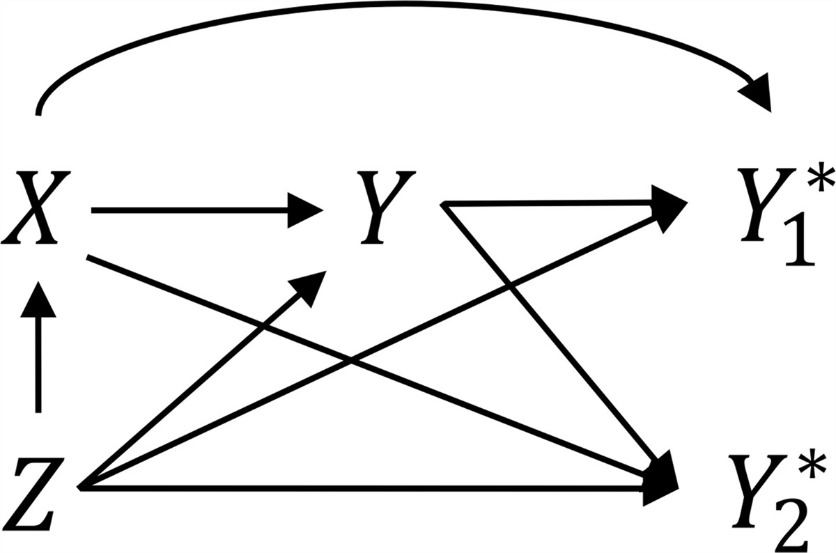
Adjusting Incidence Estimates with Laboratory Test Performances: A Pragmatic Maximum Likelihood Estimation-Based Approach

It is often of interest to estimate disease incidence. For this purpose, we typically rely on repeated measurements of participants’ disease status over time in a longitudinal framework, where disease status may be determined through lab tests. During the COVID-19 pandemic, accurate estimates of the incidence of infection with SARS-CoV-2 have been critical for public health policy decision-making.1–3 There are multiple challenges to achieving this goal that include a sub-population that is asymptomatic and a dynamic landscape of disease variants and diagnostic tests. Specifically, several SARS-CoV-2 test kits (rt-nucleic acid amplification, antigen, and serological tests) were approved under Emergency Use Authorization for clinical use without rigorous validation.4,5 The SARS-CoV-2 literature demonstrated how critical it was to adjust for the varying performance of these laboratory tests (sensitivity and specificity) to draw an accurate inference on prevalence and incidence.6,7 Indeed, for cross-sectional studies designed to estimate prevalence, the “standard correction” method based on Bayes’ rules6,8 was often applied to account for the laboratory test performance.9–13 Both frequentist8,9,14 and Bayesian approaches11–13,15 were proposed for this purpose. For example, Bajema et al.9 and Havers et al.10 proposed a two-stage nonparametric bootstrapping approach that resampled the false positive and negative cases to account for the uncertainty of the sensitivity and specificity estimates. Meireles et al.11 used a Bayesian approach with uniform prior distributions of sensitivity and specificity, whereas Sahlu and Whittaker12 considered an informative beta prior and Meyer et al.13 proposed more specific beta prior distributions that incorporated information by geographical regions. Under scenarios where knowledge of test performance was limited, Burstyn et al.16 proposed a Bayesian approach to inform the sensitivity and specificity in the population using publicly available time-series data.

Because incidence measures the instantaneous probability of being infected at a given time point, it is considered a more relevant measure for informing timely decisions on public health and healthcare resource allocation to arrest SARS-CoV-2 transmission, as it provides additional insight into the current “momentum” of the epidemic.17–20 In contrast to prevalence, incidence is often estimated with a longitudinal study design, which presents challenges in accounting for test performance.17 Given the longitudinal nature of the study required to estimate incidence, participants need to be repeatedly tested over time, yielding a high volume of tests performed. This means that even a small percentage of laboratory testing errors can result in a high absolute number of false positive or negative test results, eventually leading to a biased estimate of incidence, while the direction and magnitude of the bias would depend on the underlying true incidence and prevalence of the disease. For the purposes of our study, we defined incidence as the initial infection for a participant, where participants were censored at a positive result with no further follow-up tests scheduled. The implications of censoring as a function of the test status are that the test performance of one assay will affect whether the patient will be censored at subsequent visits, affecting the participant’s length of time considered at risk.

In the current literature, there are no guidelines or a “gold standard” approach to adjust for laboratory test errors when estimating incidence within a repeated measures longitudinal framework, which is a fairly common goal. For example, work by Becker and Britton (1999)17 and by Gan and Bain (1998)21 examined the estimation of the incidence risk under a similar longitudinal design. A key difference with the current article is our consideration of the testing error in identifying the true cases, quantified by imperfect sensitivity and specificity. Previous studies proposed methods to incorporate sensitivity and specificity by adjusting the number of positive or negative events.22,23 However, in those studies, the incidence was modeled as a single probability with only one follow-up measurement. Further, the methods proposed assumed consistent follow-up times and nondifferential time at risk and loss to follow-up across participants. Novel methods that challenged or relaxed these assumptions were proposed in the field of HIV. For example, McDougal et al.24 derived a correction factor for incidence adjustment—the probability of being infected divided by the probability of being in the window (P(T0)/P(W))—that was subsequently criticized because the correction factor took on the value of 1 under commonly occurring circumstances that did not make empirical sense.24,25 Hargrove et al.,26 therefore, proposed a modified version of a correction factor (ε)—the probability of being in the window period if infected at least twice the duration of the time interval (2μ) earlier.26 Similar to McDougal’s method, however, this approach could be misleading due to its underlying mathematical inconsistency that nonzero ε values could lead to anomalous results.25 The methods mentioned above all failed to adequately leverage the repeated nature of testing by assuming a uniform distribution of testing across all time points. Thus, there is a critical gap in the current literature for addressing unbiased estimation of incidence in a typical longitudinal framework. Flexible methods are needed that adjust for laboratory test performance in the common scenario where incidence is estimated from repeated measurements.

Parent Study: The TrackCOVID Study

Our work is motivated by a public health surveillance initiative to estimate the incidence and prevalence of SARS-CoV-2 infection and the associated risk factors in the San Francisco Bay Area (TrackCOVID study). The TrackCOVID study was conducted from July 2020 to March 2021, during the outbreak of the COVID-19 pandemic. The longitudinal study relied on a sampling framework to randomly select residents from six Bay Area counties using census tract data.27 We requested participants in the study to come into the clinic for a baseline visit and, subsequently, for monthly visits for up to 6 months. Evidence of infection was defined as a positive test using two types of assays measured repeatedly: (1) an rt-PCR test of a nasopharyngeal swab and (2) serologic testing of blood. In this way, we can capture infections that may have been missed by one of the assays, and particularly those infections we may miss in between monthly visits. Thus, our definition of infection relied on the performances of multiple assays. Importantly, to account for (1) the sampling framework, (2) the probability of selection from the household, and (3) nonresponse bias, we estimated and incorporated a combined weight variable for each participant when calculating quantities of interest (such as incidence).27

The TrackCOVID study was designated as a public health surveillance study and not human subjects research under 45 CFR 46.102(l) by the Stanford University School of Medicine Administrative Panel on Human Subjects in Medical Research and the University of California, San Francisco Institutional Review Board.

In this article, we proposed a new statistical framework to address the problem of estimating incidence while adjusting for laboratory test performance in a longitudinal repeated measures framework using a maximum likelihood estimation (MLE)-based approach. Our method can be extended to a variety of study design scenarios under relaxed assumptions. We presented the likelihood function using the motivating example, assessed the properties of the method with a simulation study, and applied our approach to the real-world data collected in our parent study.

METHODS

To better understand the underlying principles of our method, we illustrated ideas through the TrackCOVID study.

Possible Trajectories of Observed Longitudinal Test Result

In the TrackCOVID study, each participant could have at most seven visits (including the baseline visit). Considering loss to follow-up and censoring after a given visit, we may observe a total of 14 possible test result trajectories as illustrated in Table 1. For example, scenario 4 reflects the situation where an individual has three negative tests followed by a positive test at visit 4, and scenario 12 represents a trajectory where there are four consecutive negative tests immediately following enrollment with loss to follow-up afterward. In practice, observed data could be represented by either an unweighted or weighted number of participants, whose test results fall into each of these possible trajectories or scenarios, denoted as nk,k=1,⋯,14. If there is any intermittent missing value, we consider the observed data to be those preceding this value.

TABLE 1. - All Possible Trajectories of Observed Longitudinal Test Result at the Participant Level a Baseline Follow-up
Visit 1 Follow-up
Visit 2 Follow-up
Visit 3 Follow-up
Visit 4 Follow-up
Visit 5 Follow-up
Visit 6 Test result scenario 1 + Test result scenario 2 − + Test result scenario 3 − − + Test result scenario 4 − − − + Test result scenario 5 − − − − + Test result scenario 6 − − − − − + Test result scenario 7 − − − − − −− + Test result scenario 8 − − − − − − − Test result scenario 9 − Test result scenario 10 − − Test result scenario 11 − − − Test result scenario 12 − − − − Test result scenario 13 − − − − − Test result scenario 14 − − − − − −

a+ indicates a positive test result; − indicates a negative test result; and blank indicates loss to follow-up or censoring.

Possible Trajectories of True Longitudinal Infection Status

There are eight true infection status trajectories for the participants enrolled in our parent study (Table 2). Here, we assume that once a participant’s underlying true disease status is positive, their status remains positive until the last follow-up visit. Participant’s test status at each visit is a binary variable (positive or negative) that can be determined by either a single test result or multiple test results combined under prespecified rules. First, we define the following parameters:

TABLE 2. - All Possible Trajectories of True Longitudinal Infection Status at the Participant Level a Baseline Follow-up
Visit 1 Follow-up
Visit 2 Follow-up
Visit 3 Follow-up
Visit 4 Follow-up
Visit 5 Follow-up
Visit 6 Probability True status 1 + + + + + + +

q1=π

True status 2 − + + + + + +

q2=(1−π)p

True status 3 − − + + + + +

q3=(1−π)(1−p)p

True status 4 − − − + + + +

q4=(1−π)(1−p)2p

True status 5 − − − − + + +

q5=(1−π)(1−p)3p

True status 6 − − − − − + +

q6=(1−π)(1−p)4p

True status 7 − − − − − − +

q7=(1−π)(1−p)5p

True status 8 − − − − − − −

q8=(1−π)(1−p)6

a+ indicates a positive infection; − indicates no infection.

π: prevalence at baseline (probability of being infected at baseline). p: incidence at a visit assumed to be constant, (i.e., the conditional probability of infection at the current visit given no infection in the prior visit, p=P(infected at the current visit|uninfected in the prior visit)). Sen: Sensitivity (conditional probability of testing positive given infected, or P(Test +|True +)), considered fixed and as prespecified by the literature in both the parent and simulation study. Spe: Specificity (conditional probability of testing negative given uninfected, or P(Test −|True −)), considered fixed and as prespecified by the literature in both the parent and simulation study. r: the rate of loss to follow-up at a visit (conditional probability that a participant’s data are not available at the current visit given the data were observed in the prior visit).

We can express the probabilities of the eight true infection status trajectories—denoted as qi(i=1, 2, 3,…, 8)—as a function of π and p (Table 2). Note that the incidence is assumed to be constant for simplicity. Later, we extend the method to allow nonconstant incidence risk.

Likelihood Function at the Participant Level

The values of sensitivity (sen) and specificity (spe) of the laboratory test are considered to be given, and the observed data are . Given this, our interest lies in estimating (π,p). We account for test performance via the maximum likelihood estimation, which requires expressing the likelihood function. According to Tables 1 and 2, we expect to have a total of 14 × 8 = 112 combinations of the test results and the true infection status trajectories for the study cohort. We express the likelihood function for each combination as a function of π, p, and r (Tables 3 and 4).

TABLE 3. - Probability of Combination of Each Test Result and True Infection Status (True Status 1–4) True Status 1 True Status 2 True Status 3 True Status 4 Probability Test result scenario 1

sen

(1−spe)

qj

Test result scenario 2

(1−sen)sen

spesen

spe(1−spe)

(1−r^)qj

Test result scenario 3

(1−sen)2sen

spe(1−sen)sen