Negative control analyses are designed to detect bias by leveraging settings where specific causal effects are absent. Such analyses have long traditions in the basic sciences.1 For example, experimental biologists often augment their main experiment with a negative control experiment where a null effect is expected.1 If a non-null result is found in the negative control experiment, then they suspect a noncausal association between the exposure and the outcome. Thus, they would not give a causal interpretation of the result of the main experiment.1 Otherwise, if a null result is found, then the evidence for a causal effect is strengthened.

Negative control analyses have also become popular in epidemiology and are often applied to detect unmeasured confounding,1,2 selection bias,1,3,4 and measurement error.1,4,5 Furthermore, motivated by early results on negative controls, proximal inference methods have recently emerged as a rich framework for causal inference.6–8

More specifically, researchers often leverage a negative control exposure—a variable that is assumed to have no effect on the outcome variable1,4—or a negative control outcome, a variable that is assumed to be unaffected by the exposure.1,4,9 Both negative control exposures and outcomes can be used to detect bias in the main analysis.1,4,9–11 However, an alternative is to leverage a negative control population, as informally suggested in different domains of medical research.12,13 Such analyses consider a group of individuals that, informally, is assumed to be similar to the remaining population, except that the exposure has no effect on the outcome of interest through a known causal pathway. When there is no association between the exposure and the outcome in the negative control population, investigators have strengthened the argument that an exposure–outcome association in the main analysis quantifies the causal effect through the known pathway. In economics, political science, and other social sciences, the idea of negative control populations is often used in the so-called placebo population tests or placebo sample analyses.14,15 Furthermore, in these fields, negative control populations have been applied to identify average treatment effects of the treated in the presence of unmeasured confounding.15 This is possible using difference-in-difference methods if the treatment has no effect on any individual in the negative control population and if an “additive equiconfounding” assumption holds.15

In epidemiology, Davies et al.12 proposed negative control populations as a way to test the assumptions behind instrumental variable analyses and were mentioned in the reporting guidelines for Mendelian randomization studies.16 In instrumental variable settings, negative control populations are for example used to evaluate whether the exclusion restriction holds. For example, consider a genetic variant that is used as an instrument for the effect of alcohol consumption on health outcomes. In some cultures, women abstain from drinking regardless of their genetic profile, and thus they have been used as a negative control population.13,17 If no instrument–outcome association is found in women, the researcher has strengthened the argument that the genetic variant solely affects the outcome through its effect on alcohol consumption, satisfying the exclusion restriction assumption.13

While the intuition behind the use of negative control populations is ostensibly convincing, we believe that the lack of a formal definition has led to some confusion about this method. Our aim with this article is to provide an unambiguous definition of negative control populations, formalize their use to rule out unmeasured confounding and direct causal effects, and illustrate how they can be applied in epidemiologic studies.

NEGATIVE CONTROL POPULATIONS TO RULE OUT UNMEASURED CONFOUNDING

Consider the average causal effect (ACE) of a binary exposure A (A = 1 exposed, A = 0 unexposed) on an outcome Y in a population of independent and identically distributed individuals,

ACE=E(Ya=1)−E(Ya=0),

where Ya is the potential outcome had the exposure, possibly contrary to fact, been assigned to A = a.18

We will assume that the observed outcome when an individual is exposed is equal to the outcome that would have been observed in the counterfactual world in which everyone is exposed, and similarly for the unexposed. This conventional consistency18 assumption can be expressed as

Ya=YwhenA=aforalla.

Suppose that the investigator suspects confounding due to unmeasured common causes, U, of the exposure and the outcome. Suppose also that there exists a variable V such that the exposure has no causal effect on the outcome when V is equal to 1. We assume conditional positivity,18 in the sense that the probabilities of being exposed and unexposed for every level of V are strictly larger than zero, P(A=a|V=v)>0 for all a and v. To simplify the presentation, we will henceforth assume that V=0,1 is binary, but our results can be extended to settings with categorical V. Furthermore, all our results can be relaxed to be defined conditionally on baseline covariates.

We rely on the following assumption to use a negative control population.

Assumption 1 (Existence of a Negative Control Population for Unmeasured Confounding Testing)

There exists a pretreatment covariate V such that

E(Ya=1|V=1)=E(Ya=0|V=1).

Assumption 1 states that there exists a negative control group of individuals, characterized by V = 1, where the exposure has no ACE on the outcome.

Under consistency and conditional positivity, it follows that

E(Ya|A,V=1)=E(Ya|V=1)w.p.1foralla⇒E(Y|A,V=1)=E(Y|V=1)w.p.1,

where w.p.1 is short for with probability one.

In other words, when there is no unmeasured confounding in the negative control population, there is no association between A and Y in this group. Therefore, testing the null hypothesis of no exposure–outcome association in the negative control population is a valid statistical test to detect unmeasured confounding in this specific group.

Furthermore, if the exposure and the outcome are independent in the negative control population, then we will assume that there is no confounding by U in these individuals. This assumption can be formally written as follows:

Assumption 2 (No Perfect Cancelation)

E(Y|A,V=1)=E(Y|V=1)w.p.1⇒E(Ya|A,V=1)=E(Ya|V=1)w.p.1foralla.

Assumption 2 requires the absence of certain perfect cancelations. This is related to, but different from, the classical faithfulness assumptions that connect statistical (conditional) independence and the presence of directed edges in a directed acyclic graph (DAG).18–21 Assumptions 1 and 2 are immediately satisfied if the exposure has no effect on the outcome for any individual in the negative control population. Furthermore, Assumption 2 can be empirically tested in a study where the natural value of treatment is recorded just before randomization.22

Finally, we will assume that the confounding structure between the exposure and the outcome in the two strata of V is similar in the following sense:

Assumption 3 (Preserved Confounding Structure)

E(Ya|A,V=1)=E(Ya|V=1)w.p.1foralla⇒E(Ya|A,V=0)=E(Ya|V=0)w.p.1foralla.

Informally, if there is no unmeasured confounding in the negative control population, then Assumption 3 states that there is no confounding in the remaining population. Thus, we make claims about the absence of confounding in the whole population based on information about the absence of confounding in the negative control population. Assumption 3 formalizes the “similar confounding structure” notion that was used to describe the negative control population in Davies et al.12 Assumption 3 might hold even if V has strong (modifying) effects on either A or Y. Like Assumption 2, we can falsify Assumption 3 in experiments where the natural value of treatment is recorded.22

Proposition 1

Suppose consistency, conditional positivity and Assumptions 2–3 hold. If

E(Y|A,V=1)=E(Y|V=1)w.p.1

then

ACE=P(V=0).

The expression for the ACE in Proposition 1 is a g-formula.18

Suppose further that A⊥V. Then, the ACE in the overall population is equal to the marginal association between the exposure and the outcome, that is,

ACE=E(Y|A=1)−E(Y|A=0).

A formal derivation of these results is available in eText 1; https://links.lww.com/EDE/C121. Proposition 1 does not put restrictions on the dimension of U.

Analogous to classical negative control methods, we have used a null association in one analysis to corroborate the causal interpretation of the association obtained in another analysis. In practice, we would assess (test) whether E(Y|A=1,V=1)=E(Y|A=0,V=1) in our observed data. If the equality is rejected, then we will suspect bias in the main analysis. If the equality is plausible, then the argument for a causal interpretation of the main analysis is strengthened.

NEGATIVE CONTROL POPULATIONS TO RULE OUT UNMEASURED CONFOUNDING AND DIRECT EFFECTS

Suppose now that there exists a subgroup where the exposure has no effect on the outcome through a known causal pathway. For example, we know that an antibiotic has no effect on severe symptoms in individuals with viral infections through its pharmacologic action. Yet, it is possible that individuals with a viral infection fail to satisfy Assumption 1 because taking the antibiotic could still give placebo responses or lead to behavioral changes.23

Now we will modify the assumptions from the previous section and suggest a procedure to rule out both unmeasured confounding and the presence of a direct effect, that is, an effect outside of the known causal pathway. We will also revisit these results later in the manuscript and consider a relevant special case, where we suggest a test for the presence of placebo effects in unblinded randomized controlled trials.

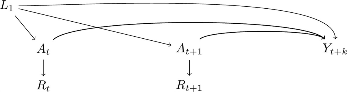
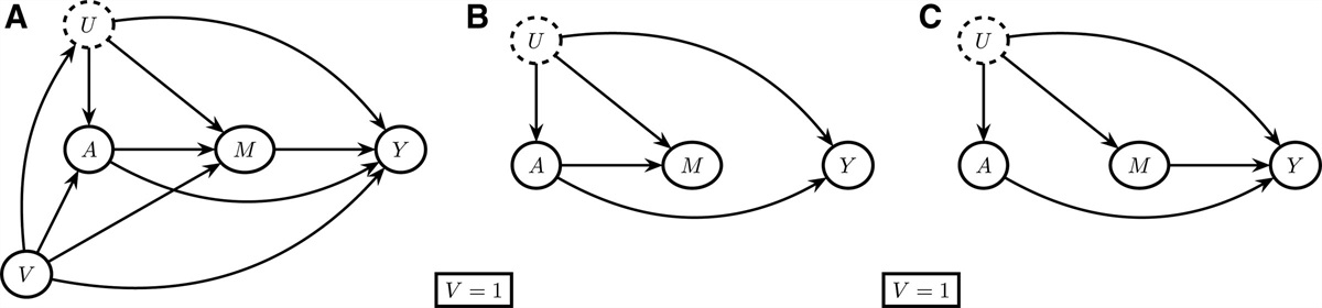
Consider a data generation process compatible with the DAG in Figure, part A. The variable M represents a known mediator variable of the effect of the exposure on the outcome, and U represents all common causes of A, M, Y, or any pair of these variables. To simplify the exposition, we will assume that P (Y = y, M = m, A = a, U = u, V = v) > 0 for all y, m, a, u, v in the remainder of this section. There are two potential causal pathways from the exposure to the outcome, a direct path (A→Y) and a path that goes through M (A→M→Y). We will modify Assumption 1 in the sense that the negative control population will be defined with respect to indirect effects through M; informally, the negative control population is now a population where the treatment is only known to exert no effects through M.

FIGURE.:

Directed Acyclic Graph. A, shows a directed acyclic graph representing causal relationships between the exposure (A), the mediator (M), the outcome (Y), the unmeasured common cause (U), and the variable indicating the negative control population (V). B and C, show conditional directed acyclic graphs in two possible scenarios where the exposure has no effect on the outcome through the mediator.

Assumption 4 (Existence of a Negative Control Population for Confounding and Direct Effect Testing)

Suppose that one of the following two statements holds:

4a.P(Ma=1=m|U,V=1)=P(Ma=0=m|U,V=1)w.p.1forallm

4b.E(Y|M,A,U,V=1)=E(Y|A,U,V=1)w.p.1.

In a negative control population satisfying Assumption 4, the exposure has no effect on the mediator conditioning on the unmeasured variable U (4a), or the mediator is independent of the outcome conditional on U and A (4b) in this subgroup. Conditional DAGs can be useful to visualize Assumption 4, because this assumption only involves one level of V. Two conditional DAGs compatible with 4b (panel B) and 4a (panel C) are given in Figure.

When there is no unmeasured confounding and no direct effect in the negative control population, E(Y|A=1,V=1) and E(Y|A=0,V=1) are the same, see eText 1; https://links.lww.com/EDE/C121 for a more formal statement. Therefore, testing for the null hypothesis of equality of these two quantities is a valid statistical test for detecting the presence of unmeasured confounding or direct effects in this subgroup.

Similar to Assumption 2, we will assume no perfect cancelation for the direct effect.21

Assumption 5 (No Perfect Cancelation of Direct Effects)

E(Y|A,V=1)=E(Y|V=1)w.p.1⇒E(Ya=1|Ma=1=m,U,V=1)=E(Ya=0|Ma=0=m,U,V=1)w.p.1.

for all m. When A and Y are independent in the negative control population, then Assumption 5 requires that there is no direct effect of A on Y in this subgroup.

Assumptions 4b and 5 could alternatively be expressed in terms of no causal effect of M on Y and no controlled direct effect of A on Y when M is fixed. Unlike our formulation of Assumptions 4–5, these alternative representations would require us to explicitly consider an intervention on M, but would not require us to explicitly include U in these statements.

We also assume that, unlike the indirect effect, there is no context-specific direct effect in the following sense.

Assumption 6 (No Context-specific Direct Effect)

E(Ya=1|Ma=1=m,U,V=1)=E(Ya=0|Ma=0=m,U,V=1)w.p.1forallm

⇒E(Ya=1|Ma=1=m,U,V=0)=E(Ya=0|Ma=0=m,U,V=0)w.p.1.forallm.

Assumptions 5 and 6 imply that if E(Y|A=1,V=1)=E(Y|A=0,V=1), then there is no direct effect of the exposure on the outcome. If Assumptions 2 and 3 also hold, then the ACE is a simple function of observable quantities and, informally, it represents the effect of A on Y through M.

Assumptions 2 and 5 are only plausible when V is temporally ordered before A and U. If not, then conditioning on V might introduce a noncausal association between the exposure and the outcome, that is, a collider bias.18 Because of the collider bias, the existing informal definition of a negative control population12 might be misleading. Inspired by the Mendelian randomization literature,13,17,24–26 we discuss this issue in a study evaluating the effect of alcohol consumption on health outcomes in eText 2; https://links.lww.com/EDE/C121. In this example, we also show that our results hold under weaker positivity assumptions, such as when certain deterministic relationships exist between V and M.

NEGATIVE CONTROL POPULATIONS ARE RELEVANT TO EPIDEMIOLOGISTS

Consider an observational study comparing the effect of two wide-spectrum antibiotic treatments on mortality in patients with sepsis. As usual, the antibiotics were administered based on symptoms and initial laboratory tests, while waiting for the confirmatory results from the bacteria cultures. However, after a few days, the culture tests showed that a subgroup of patients was affected by a strain that is resistant to the antibiotics under investigation. The individuals affected by the resistant strain could satisfy our criteria for a negative control population since we expect no effect of a known mediator (antibacterial agent intake) on the outcome among these patients (Assumption 4b).

Consider also a study that evaluated the effect of initiating a prophylactic HIV treatment on mortality in a population of HIV-negative individuals. It is known that some humans have innate resistance to HIV.27 These individuals could be included in the trial because the resistance status was unknown at the time of study recruitment. While the study was ongoing, the investigators performed a new genetic test and detected the immunity status in a subgroup of the participants.28 This subgroup would satisfy our assumptions of a negative control population since the treatment has no effect on a known mediator (HIV infection) among these individuals (Assumption 4a).

The two examples illustrate that negative control population methodology is suitable when some individuals have a characteristic, such as an infection by a resistant microbe or a genetic predisposition, that makes them immune to a condition.

More broadly, negative control population methodology is appropriate when studying policies15 and what we denote as suboptimal interventions. These interventions are implemented due to their convincing average effects, even if a (small) proportion of individuals are unaffected by the intervention through the mechanism that justified its implementation. The term “sub-optimal” is not meant to insinuate that initiating the intervention is wrong or undesirable; we merely emphasize that a subgroup of individuals will not benefit from the intervention in the intended way. At treatment initiation, these subgroups can indeed be impossible to detect. Nevertheless, we can use the subgroups in later negative control analyses, as we illustrate in the next example.

THE EFFECTS OF MOBILE STROKE UNITS ON FUNCTIONAL OUTCOMES

Mobile stroke units (MSUs) are ambulances designed for prehospital management of stroke patients.29 Unlike standard ambulances, these units are equipped with a computed tomography (CT) scanner, point-of-care laboratory testing, telemedicine connection to stroke centers, and specifically trained personnel.30,31 The main purpose of the MSU is to shorten the time from onset of cerebral ischemia to thrombolytic treatment.29 This is important because the effect of thrombolysis decreases considerably with time.32 However, thrombolysis is only effective in patients with cerebral ischemia and should not be administered to patients with other diagnoses or stroke patients with contraindications to thrombolytic treatment, for example, because of a hemorrhagic stroke. Ischemic and hemorrhagic stroke patients are symptomatically indistinguishable and a CT scan is needed to correctly diagnose them. Because CT scans are performed in MSUs, thrombolytic treatment can be initiated already in the prehospital phase, which shortens the time from stroke onset to thrombolysis for eligible patients.30,33 Large controlled studies found that additional dispatch of MSU has a beneficial effect on outcomes in ischemic stroke patients31,33–35 and, in 2022, MSU management was suggested by the European Stroke Organisation guidelines to improve stroke prehospital management.30

We applied the negative control population methodology to data from the “Benefits of Stroke Treatment Delivered by a Mobile Stroke Unit Compared with Standard Management by Emergency Medical Services” (BEST-MSU) trial.31 The main analysis of the BEST-MSU concerned the effect of MSU dispatch on functional outcomes after 3 months among patients without contraindication to thrombolysis. We provided a short description of the study design in eText 3; https://links.lww.com/EDE/C121.

We emphasize that the BEST-MSU did not randomize individuals to MSU treatment or standard ambulance; the treatments were sequentially assigned to all participating sites in different time periods. While this design should mitigate confounding, the investigators were nevertheless concerned about the possibility of this type of bias. Thus, the BEST-MSU trial reported secondary analyses where inverse probability of treatment weighting was used to adjust for measured confounders, such as study site, baseline stroke severity, prestroke functional outcome, age, ethnicity, sex, and time from last seen well to ambulance arrival.31

Rather than leveraging the measured covariates, we relied on a negative control population to assess whether the MSU analysis was biased. Our question of interest was the effect of additional MSU dispatch on functional outcome at hospital discharge, among all enrolled patients, that is, regardless of the subsequent thrombolysis eligibility assessment. The outcome was specifically defined as a utility-weighted version of the modified Rankin scale (mRS) assessed at hospital discharge, used by the BEST-MSU researchers as a measure of the functional outcome.31 The average utility-weighted mRS for each level of the mRS is publicly available,31 and we used this information to approximate the continuous outcome. We extracted the data about the mRS distribution by dispatch group, separately for enrolled patients without hemorrhagic stroke or stroke mimic diagnosis (ischemic patients) and for the enrolled patients with these diagnoses (other patients), from the Supplementary Material of the original BEST-MSU study (see Table).31

TABLE. - Modified Rankin Scale (mRS) and Utility-weighted Modified Rankin Scale (uw-mRS) by Dispatch Group Are Presented for Ischemic Patients and Other Patients, Comprising Hemorrhagic Stroke and Stroke Mimic Variables Ischemic Patients (N = 1,103) Other Patients (N = 412) Overall (N = 1,515) Conventional Ambulance (N = 452) MSU (N = 651) Conventional Ambulance (N = 177) MSU (N = 235) mRS N-Miss 0 0 0 1 1 0 38 (8%) 126 (19%) 13 (7%) 27 (12%) 204 (13%) 1 91 (20%) 123 (19%) 26 (15%) 34 (15%) 274 (18%) 2 71 (16%) 82 (13%) 13 (7%) 30 (13%) 196 (13%) 3 78 (17%) 109 (17%) 27 (15%) 25 (11%) 239 (16%) 4 92 (20%) 124 (19%) 51 (29%) 54 (23%) 321 (21%) 5 64 (14%) 68 (10%) 35 (20%) 47 (20%) 214 (14%) 6 18 (4%) 19 (3%) 12 (7%) 17 (7%) 66 (4%)