Administrative population registers play a vital role in epidemiology, providing data on disease incidence and exposure across more or less entire populations.1 However, despite their richness in data, these databases can have shortcomings such as incomplete coverage, data inaccuracies, and absent records. For instance, it is often unclear if the data source(s) used to measure outcomes can capture all relevant outcome events. Unlike studies with original data collection, where researchers are typically aware of which individuals have missing data, unrecorded events in register-based studies lead to a problem called “under-ascertainment.”2 This issue arises from our inability to differentiate between individuals with missing outcomes and those without, which means that conventional missing data imputation cannot be employed.

Under-ascertainment leads to an underestimation of disease prevalence and incidence and can therefore hamper disease surveillance efforts. When outcome ascertainment depends on individual characteristics, it can also result in biased exposure (or treatment) effect estimates by biasing the observed outcome numbers downward in one group more than the other, compromising the validity of causal estimates in a way similar to confounding.1,3 Despite these serious implications, under-ascertainment often goes unaddressed in empirical studies.4

Researchers often conduct register validation studies to assess the accuracy of disease classifiers by comparing them with gold standard reference data, which are presumed to be complete.1,4 In situations where such reference data are unavailable, capture–recapture methods can be employed. These methods use imperfect case data from multiple sources to estimate the true prevalence of underreported diseases.5–10 For example, techniques have been applied to uncover “hidden” public health challenges such as drug use,11 modern slavery,12 homelessness,13 and more.14 However, existing capture–recapture methods have not been developed to estimate exposure effects, limiting their value for epidemiologic research.

In this paper, we introduce an ascertainment probability weighting (APW) framework that combines capture–recapture with exposure propensity scores to simultaneously address under-ascertainment and confounding. Unlike existing empirical approaches for handling outcome misclassification, which require a single, perfect validation dataset, our approach exploits outcome data from two imperfect sources.15–25 We begin by introducing our framework and estimator, highlighting the assumptions required for valid estimation. We then demonstrate the approach through a hypothetical example and an empirical case study on under-ascertained coronavirus disease 2019 (COVID-19) tests in Sweden, while providing practical implementation guidance, discussing strengths and limitations, and highlighting its appropriate usage scenarios.

METHODS Preliminaries and Notation

This section introduces the notation used throughout the paper. Let Yi denote a binary “target outcome” of interest, such as disease outcomes (e.g., lung cancer), health behaviors (smoking), or other characteristics (being homeless). Xi represents a predictor of interest (e.g., an exposure or treatment variable), and Zi represents covariate(s).

To be concise, we often employ shorthand expressions when presenting conditional probabilities. For instance, instead of writing out the full expression P(Xi=x|Zi=z), we write P(x|z).

Under-ascertainment

Our framework addresses under-ascertainment, a type of one-sided outcome misclassification. Under-ascertainment occurs when individuals with Yi=1 may either be correctly classified as Yi∗=1 or wrongly classified as Yi∗=0, but all individuals with Yi=0 are always classified correctly as Yi∗=0 (i.e., there are no false positives). In the machine learning literature, this is often referred to as a positive-unlabeled classification problem.26

Causal Framework and Assumptions

To relate the realized Yi to causal estimands, we apply the potential outcomes framework.27 This framework defines a potential outcome Yi(x) as the outcome that would occur if the exposure (or treatment), perhaps contrary to fact, were set to x. We assume standard causal assumptions: consistency (Yi=Yi(x) whenever Xi=x is observed), exchangeability of Xi and the potential outcomes conditional on observed covariates Zi (Yi(x)⊥Xi|Zi for all x), and exposure positivity (P(x|z)>0 for all x and z). We also assume that all variables except Yi are measured without error, and that the study sample is representative of the (super-)population of interest.

Ascertainment Probability Weighting

Our objective is to estimate P(Yi(x)=1), representing the potential outcome probability under exposure level x, which can be used to compute various marginal causal effects, such as risk differences (RDs) or risk ratios (RRs).

In Equation (A4) in the Appendix, we establish a relationship between P(Yi(x)=1) and the under-ascertained data according to the following expression:

P(Yi(x)=1)=∑zP(Yi∗=1,x|z)P(z)P(Yi∗=1|Yi=1,x,z)P(x|z).

Here, P(Yi∗=1|Yi=1,x,z) is the ascertainment probability conditional on x and z. The rest of the expression follows the principles of conventional inverse probability weighting (IPW), including adjustment for confounding by inclusion of the exposure propensity score, P(x|z), in the denominator, which adjusts for observable confounders (Zi) by balancing their distribution between exposure groups.28 For continuous Zi, the summation can be replaced by integration.

Although Equation (1) cannot be computed directly due to the unobserved nature of Yi, it can be estimated using capture–recapture. In our data setup, we observe under-ascertained outcome data from two data sources, where Yji∗=1 indicates the outcome’s ascertainment in source j∈. In turn, Yi∗=1 means that the outcome has been ascertained in at least one source, that is, Yi∗=1 if Y1i∗=1 or Y2i∗=1.

We make two core assumptions beyond those mentioned in the previous section.

Assumption 1 (conditional source independence).Y1i∗⊥Y2i∗|(Yi=1,Xi,Zi).Assumption 1 means that we assume conditional independence of the probability of ascertainment between the two data sources, given Yi=1 and observed characteristics Zi and Xi. This relaxation of the basic capture–recapture method’s marginal independence assumption, which has also been exploited by others (e.g., Das et al.,7 Alho,8 and Tilling and Sterne9), is akin to the conditional exchangeability assumption with respect to exposure, used for causal estimation in observational studies when adjusting for confounding by observed covariates. In practice, the covariates involved should correspond to factors that are correlated with ascertainment in both sources, such as geographical factors and health behaviors.
Assumption 2 (ascertainment overlap).P(Y1i∗=1,Y2i∗=1|Yi∗=1,x,z)>0 for all (x,z).Assumption 2 means we assume a positive probability for ascertained cases to appear simultaneously in both data sources within all strata of Xi and Zi. This condition is analogous to the exposure positivity assumption and can be verified by examining whether at least some ascertained cases are observed in both sources within all covariate strata.

If Assumptions 1 and 2 hold, Proposition 1 from Das et al.7 shows that

P(Yi∗=1|Yi=1,x,z)=P(Y1i∗=1,Y2i∗=1|Yi∗=1,x,z)P(Y1i∗=1|Yi∗=1,x,z)P(Y2i∗=1|Yi∗=1,x,z).

The right-hand side of Equation (2), which reflects capture–recapture-derived ascertainment probabilities, depends solely on probabilities within the subpopulation with Yi∗=1 (see Appendix Equations (A1–A3)). Consequently, it can be estimated from observable data. Substituting the right-hand side of Equation (2) into Equation (1), we have that

P(Yi(x)=1)=∑zP(Yi∗=1,x|z)P(z)P(Y1i∗=1,Y2i∗=1|Yi∗=1,x,z)P(Y1i∗=1|Yi∗=1,x,z)P(Y2i∗=1|Yi∗=1,x,z)P(x|z).

This formulation allows us to apply APW using capture–recapture methods, providing a practical solution for handling under-ascertainment while estimating causal effects.

Estimation

Equation (3) provides an avenue for estimation using a plug-in estimator. In the Appendix (Equation (A5)), we also derive the following estimator to simplify estimation with individual-level data:

P^(Yi(x)=1)=1N∑Ni=1I(Yi∗=1,Xi=x)P^(Y1i∗=1,Y2i∗=1|Yi∗=1,xi,zi)P^(Y1i∗=1|Yi∗=1,xi,zi)P^(Y2i∗=1|Yi∗=1,xi,zi)P^(x|zi).

This estimation approach simplifies the process by avoiding the need to parametrically estimate the numerator. In Equation (4), N represents the size of the study sample, and I(Yi∗=1,Xi=x) is an indicator function coded as 1 for individuals with observed Yi∗=1 and whose observed exposure Xi is equal to x, and 0 otherwise. The remaining terms represent predicted probabilities for each individual i, which can be obtained either through nonparametric methods or parametric techniques, such as logistic regressions. Naturally, the consistency of the estimator hinges on these models being correctly specified.

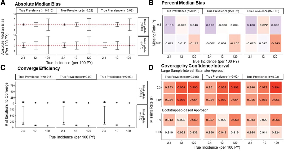
eAppendix 1; https://links.lww.com/EDE/C109 contains a simulation validating the estimator’s performance when all assumptions are met. The simulation also verifies that percentile-based bootstrap confidence intervals, derived from resampling the full size, N study sample with replacement, can be used to quantify the uncertainty of APW estimates (eAppendix 1; https://links.lww.com/EDE/C109).

Numerical Example

To aid intuition about the method, we first present a hypothetical example focusing on the association between seatbelt use and injury risk in car crashes. In eAppendix 2; https://links.lww.com/EDE/C109, we also provide code to generate similar data and show how the method can be applied with individual-level observations.

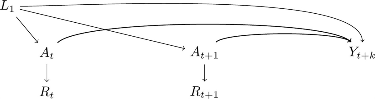
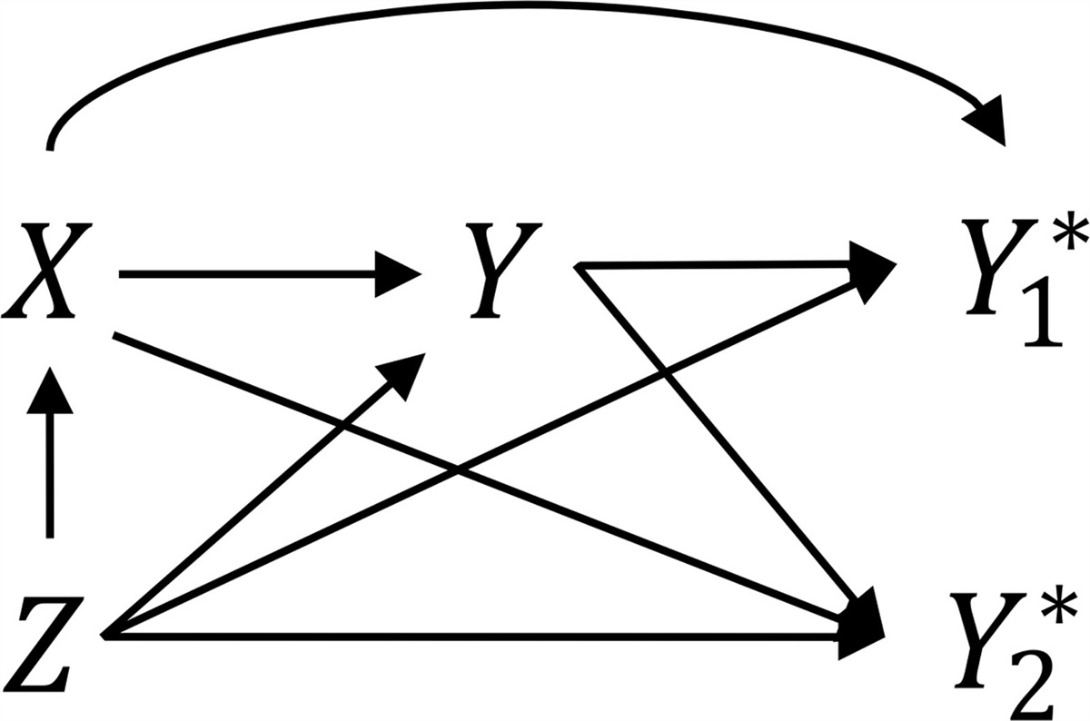
Our hypothetical data follows the causal model in the Figure. The observed outcome data, Yi∗, are gathered from two sources: police records, Y1i∗, and hospital admissions, Y2i∗. The unit of observation is car crash events, where injury outcomes are imperfectly ascertained. In our data-generating process, confounding bias arises from drunk driving (Zi), which is a common cause affecting both seatbelt use (Xi) and the true injury outcome (Yi). Under-ascertainment bias occurs because both Xi and Zi impact ascertainment in the two data sources. Specifically, seatbelt use affects injury likelihood and severity, which, in turn, influence ascertainment in both police and hospital records. Additionally, drunk driving may affect the likelihood of police ascertainment of injury outcomes for all involved parties, as well as influence injury and crash severity. Consequently, under-ascertainment varies across the four strata defined by Xi and Zi.

FIGURE.: Directed acyclic graph depicting the causal model used to generate the hypothetical example data. In our hypothetical example, Y stands for car crash injury, X is seatbelt use, and Z is drunk driving. Our exposure of interest is X and Z is a confounding variable (a common cause of X and Y). The true Y is unobserved; instead, we observe under-ascertained outcomes from two sources, represented by

Y1∗

(police records) and

Y2∗

(hospital admissions data). Seatbelt use and drunk driving (X and Z) each affect the probability of ascertainment in both sources, as depicted by the arrows from these variables into

Y1∗

and

Y2∗

.

Table 1 contains conditional probabilities based on a scenario such as the one outlined above. Setting P(Zi=1) to 0.5 for simplicity, the potential outcome probabilities P(Y(1)=1) and P(Y(0)=1) in the population are 0.379 and 0.621, respectively. The true causal RD is therefore −0.242, and the causal RR is 0.61. Estimating these effects using the observed Yi∗, we instead get −0.099 for the RD and 0.76 for RR, which are both clearly biased. These estimates are already adjusted for confounding by Zi, so the bias is solely related to differential ascertainment.

TABLE 1. - Conditional Probabilities From a Hypothetical Register-based Study Suffering From Outcome Under-ascertainment With Imperfect Outcome Data From Two Sources Variable Values Conditional Probability X = 1, Z = 1 X = 1, Z = 0 X = 0, Z = 1 X = 0, Z = 0 Outcomes  

P(Yi(x)=1x,z)

a,b 0.449 0.309 0.691 0.550  

P(Yi∗=1x,z)

0.411 0.215 0.552 0.272  

P(Yi∗=1,xz)

0.256 0.082 0.208 0.169 Exposure propensities  

P(xz)

0.623 0.379 0.377 0.621 Ascertainment  

P(Yi∗=1Yi=1,x,z)

a,c 0.917 0.698 0.797 0.494  

P(Y1i∗=1Yi∗=1,x,z)

0.751 0.648 0.688 0.627  

P(Y2i∗=1Yi∗=1,x,z)

0.799 0.643 0.689 0.539  

P(Y1i∗=1,Y2i∗=1Yi∗=1,x,z)

0.550 0.291 0.378 0.167

aThese conditional probabilities (and their sample analogues) are presumed to be unobservable in our data setup but are displayed here for reference.

b

P(Y(x)=1)=∑z⁡P(Yi(x)=1x,z)P(z)

gives the marginal potential outcome probabilities. We apply this formula to compute the true RD and RR and use the same method on

P(Yi∗=1x,z)

to obtain the biased RD and RR presented in the text.

cTrue ascertainment probabilities. These are unobservable but estimable from observable data by capture–recapture methods using Equation (2). For instance, plugging the three observable ascertainment probabilities from the left-most column into the equation gives us 0.550/(0.751 × 0.799) ≈ 0.917, which is equivalent to the true ascertainment probability.

To address the remaining bias, we first apply Equation (3) to estimate P(Yi(1)=1):

P(Yi(1)=1)=∑z⁡P(Yi∗=1,Xi=1|z)P(z)P(Y1i∗=1,Y2i∗=1|Yi∗=1,Xi=1,z)P(Y1i∗=1|Yi∗=1,Xi=1,z)P(Y2i∗=1|Yi∗=1,Xi=1,z)P(Xi=1|z)=0.256×