A Quantitative Bias Analysis Approach to Informative Presence Bias in Electronic Health Records

Electronic health records (EHRs) are a key data resource for clinical research. While EHRs have advantages such as capturing a more representative patient sample than clinical trials and including rich data on the entire care process,1 the availability of patient-level data, which is collected during care, can vary substantially. Importantly, such variation is usually not random and is often driven by factors such as health status. For example, compared with a patient with lower comorbidity burden, a patient with higher comorbidity burden may have more complete data recorded in the EHR, since comorbidity is associated with more interactions with the health care system.2–4 The data collection process, which corresponds to the visit process in the EHR context, is considered informative in that it reflects patient characteristics such as health status.

Ignoring informative visit processes can lead to bias in EHR-based analyses. For example, consider two independent conditions X and Y. If condition X substantially increases the visit frequency, it is likely to appear that X is associated with a higher risk of Y, because patients with X have more clinical encounters at which diagnosis codes or other indicators of Y can potentially be captured, compared with those without X. When assessing such an association between two conditions, conditioning on the visit frequency has been found to mitigate this bias.5,6 However, conditioning can introduce a new source of bias, collider bias, if the visit frequency is impacted by both underlying conditions. Even when the visit frequency is not a collider, conditioning may not fully remove bias due to informative observation.6 Therefore, quantitative bias analyses exploring robustness of results to assumptions about the structure and magnitude of potential misclassification may be useful.

This article aims to extend previous work on informative presence bias by assessing the utility of a quantitative bias analysis method for misclassification. Validity of the quantitative bias analysis method was assessed using simulation studies and benchmarked against bias resulting from a naïve method ignoring misclassification and a method conditioning on visit frequency. We characterize the performance of these approaches in the context of alternative structures for the dependence of misclassification on visit frequency.

MOTIVATING EXAMPLE

Consider using an oncology EHR database to assess the relationship between diabetes and cancer progression or death in patients with metastatic breast cancer. EHR data may not accurately reflect the true status of diabetes, cancer progression, or death, leading to potential misclassification that can bias the estimate of the association. A patient who truly has either condition may have no record indicating a diagnosis of the condition (EHR-derived phenotype with imperfect sensitivity) because they had few or no clinical encounters during the study period; it is also possible for a patient who truly has neither condition to have a record indicating a diagnosis (phenotype with imperfect specificity) due to lack of specificity of diagnosis codes or erroneous EHR data.

Prior research suggests that EHR-derived comorbidity may be inaccurate.7 An oncology EHR-derived diabetes phenotype may be even less accurate, since data outside the oncology care setting may be unavailable.8 An oncology EHR-derived progression or death phenotype may also be imperfect. While EHR-based capture of mortality has been demonstrated to have good sensitivity and specificity,9 using EHR data to accurately capture progression remains challenging. Progression is defined based on the Response Evaluation Criteria in Solid Tumors in clinical trials, but ascertaining real-world progression relies on clinicians’ notes, and a Response Evaluation Criteria in Solid Tumors-based real-world progression phenotype has remained infeasible.10 Moreover, in routine practice, patients may not be evaluated at regularly scheduled fixed intervals resulting in differential ascertainment of time to progression across patients.

Further complicating the issue, the extent of misclassification in the exposure (or outcome) may vary by the true outcome (or exposure) status, due to the informative visit process. Because diabetes may be associated with more frequent visits,11 those with diabetes may have more complete data facilitating more accurate classification of the status of progression. Similarly, progression may be associated with more frequent visits in the preceding period, providing more complete data for classification of diabetes status. Such relationships will result in informative presence bias in the estimate of the association of interest. The estimate may be biased even when the study population is restricted to those having at least some minimum visit frequency, as has been previously proposed to ensure acceptable data quality.12–14 Moreover, the resultant selected population may no longer be representative.

CONCEPTUALIZATION

Let X and Y denote diabetes and progression or all-cause death, respectively. For ease of description, X is referred to as the exposure of interest and Y the outcome. Both X and Y are defined as binary variables, which take the value of 1 if a patient ever experienced the condition during study period and 0 otherwise. We assume the underlying outcome model is the log-binomial model, and the target of inference is the relative risk describing the association between X and Y. The log-binomial model is assumed because it is collapsible, ensuring that bias in log-relative risk estimates is not due to noncollapsibility. We assume that assessment of both X and Y relies on EHR data: if there is at least one record during the study period indicating a diagnosis of X (or Y), then the observed exposure (or outcome), denoted XO (or YO), takes the value of 1; otherwise, XO=0 (or YO=0). We refer to XO and YO as EHR-derived phenotypes. Let N denote the visit frequency, with N=1 representing frequent visitors and N=0 representing infrequent visitors. Specific intensity of encounters that would be considered “frequent” or “infrequent” will be context specific and relates to the probability that a condition is captured if a visit is made as well as the rate of evolution of the condition. Neither the frequent nor the infrequent visitors include individuals who never visit the health care system, since they typically cannot be captured by an EHR database. We additionally assume the presence of a confounder Z that has a direct effect on X, Y, and N. Except for X and Y, all other variables are assumed to be perfectly measured.

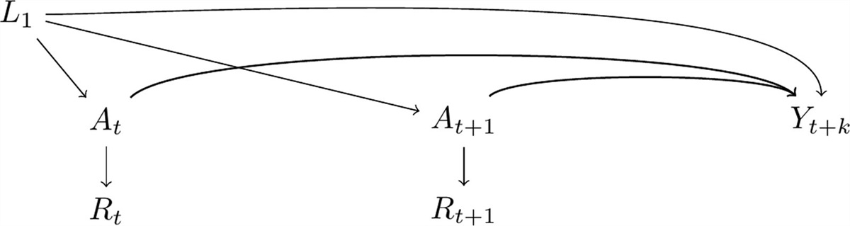
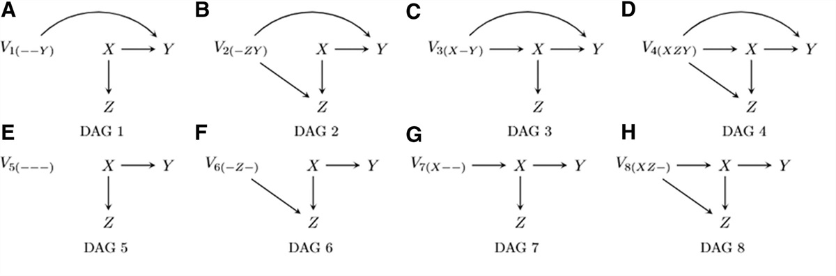
Hernán and Cole15 classified exposure and outcome measurement error into four types, depending on whether the measurement error is nondifferential or whether it is independent. When both the exposure and outcome are binary, as in the current study, measurement error takes the form of misclassification. The misclassification in X (or Y) is considered nondifferential if XO (or YO) is independent of Y (or X). In the motivating example, nondifferential outcome (or exposure) misclassification occurs if the EHR-derived progression or death (or diabetes) phenotyping accuracy is the same for patients with or without diabetes (or progression or death). The misclassifications in X and Y are considered independent of each other if XO and YO are independent, conditional on X and Y. In the motivating example, independent misclassification occurs if EHR-derived progression or death (or diabetes) phenotyping accuracy is the same for patients with or without correctly classified diabetes (or progression or death) status. Therefore, we considered four classes of possible data-generating mechanisms that lead to exposure and/or outcome misclassification, depicted in Figure 1 (A1–4: nondifferential independent; B1: nondifferential dependent; C1–4: differential independent; D1–3: differential dependent). All misclassification structures in Figure 1 assume dependence of X and Y on Z.

FIGURE 1.: Directed acyclic graphs representing exposure and outcome misclassification structures. A, Nondifferential independent (conditional on Z)a. B, Nondifferential dependent (conditional on Z)a. C, Differential independent (conditional on Z)a. D, Differential dependent (conditional on Z)a. aA misclassification structure is considered nondifferential if, after conditioning on

Z

, the misclassification in ? (or ?) is independent of ? (or ?); otherwise, the misclassification is considered differential. A misclassification structure is considered independent if, after conditioning on

Z

, the misclassification in ? (or ?) is independent of the misclassification in ? (or ?); otherwise, the misclassification is considered dependent.

In settings where differential and/or dependent misclassification is present, conditioning on the visit frequency N can mitigate bias by converting the original misclassification structure into one that is conditionally nondifferential and independent.6 Nonetheless, bias may not be completely removed by conditioning on N, as bias toward the null due to nondifferential independent misclassification will persist. Additionally, when N is directly impacted by X and Y (Figure 1, C3, C4, and D3), conditioning on N induces collider bias.

Lyles and Lin16 proposed a quantitative bias analysis method for misclassification. When only the binary exposure (or outcome) is subject to misclassification, each observation is first replaced by two observations representing both possible true values of the underlying exposure (or outcome). Each of the new observations is then weighted using positive and negative predictive values, which are estimated based on assumed sensitivity and specificity along with the observed data. This approach seeks to create a misclassification-free pseudo-population. Standard errors may be estimated via jackknifing or bootstrapping.

Lyles and Lin16 also provided extensions that accommodate situations where more than one variable is subject to misclassification. In the current setting, both X and Y are subject to misclassification; upon conditioning on the visit frequency N, the misclassification in each variable is independent of the other. To implement the quantitative bias analysis method, each original observation (XO, YO, N, Z) is replaced by all four possible combinations of the true, unobserved values of X and Y, along with the N and Z values as observed. Each record is weighted by the probability of X and Y conditional on XO, YO, N, and Z, which is estimated based on assumed sensitivity and specificity (for both X and Y among frequent and infrequent visitors, respectively) and the observed data (eAppendix 1; https://links.lww.com/EDE/C116). A weighted log-binomial model is then fit in the expanded dataset, with Y as the outcome, and X and Z as covariates. Because this method directly adjusts for misclassification, it can fully remove bias without risking inducing collider bias if the sensitivity and specificity are correctly specified. In realistic situations where the true sensitivity and specificity are unknown, a series of quantitative bias analyses may be conducted to evaluate robustness of results over a grid of plausible values.

SIMULATION STUDY Simulation Setup

We conducted simulation studies to investigate bias in estimated log-relative risks in the presence of visit-dependent exposure and/or outcome misclassification. We considered three analytical approaches: (1) a naïve approach ignoring misclassification, (2) an analysis conditioning on visit frequency, and (3) using predictive value weighting as described above. We investigated each misclassification structure in Figure 1 when X and Y are independent and when X and Y are associated, respectively.

For a sample of 5000 patients, we first generated a confounder Z from a normal distribution (mean = 60, standard deviation = 10). We assumed the confounder Z to directly impact the binary exposure X, the binary outcome Y, and the visit frequency N. Specifically, we generated X using a logistic model:

logit(P(X=1|Z))=βX0+βXZ(Z−Z¯).

We then generated Y from a Bernoulli distribution with probability

log(P(Y=1|X,Z))=βY0+βYXX+βYZ(Z−Z¯).

We subsequently generated N following a logistic model:

logit(P(N=1|X,Y,Z))=βN0+βNXX+βNYY+βNZ(Z−Z¯).

We varied coefficients depending on the specific misclassification structure (Table 1). Across all misclassification structures, the baseline prevalences of X, Y, and frequent visitors were approximately 50%, 20%, and 20%, respectively.

TABLE 1. - Simulation Parameters for Different Misclassification Structures Structure

βX0

βXZ

βY0

βYX

βYZ

βN0

βNX

βNY

βNZ

X sen (

N=0