A primary goal of many epidemiologic studies is estimation of the causal risk difference (or a similar causal estimand). Investigators typically focus on point identification of causal risk differences under strong unverifiable assumptions, for example, under assumptions of conditional exchangeability, consistency, and positivity. However, it is also possible to partially identify or bound causal effects, meaning we can identify upper and lower limits on the possible magnitude and direction of effect. This can be done using the data and consistency alone, without assumptions about the data-generating mechanism.1,2 Previous studies have called for the incorporation of these upper and lower limits, known as assumption-free bounds, into more epidemiologic studies.3–6 Previous epidemiologic descriptions of “assumption-free” bounds have focused exclusively on point interventions. Here, we describe simple expressions for assumption-free bounds for the causal effect of static and dynamic sustained treatment regimes. We also highlight the connection between the assumption-free bounds and “clone-censor-weight” methods.7,8 This connection allows for easy calculation of the assumption-free bounds in practice and gives intuition about factors influencing the width of the assumption-free bounds.

ASSUMPTION-FREE BOUNDS FOR BINARY TIME-FIXED TREATMENTS

For a binary outcome Yk+1 at some time k + 1, the causal risk difference comparing two levels of an exposure Ak is naturally bounded between −1 and 1 without looking at any data at all. However, when data are available, we can narrow bounds on causal effects under consistency, which allows us to connect counterfactuals, which we denote with superscripts Yk+1ak, to observed data. For each individual i in a population, consistency is formally stated as “if Ai,k=ai,k, then Yi,k+1=Yi,k+1ak.” Informally, this means that the counterfactual treatments are well-defined and correspond to the versions in the data.

Using consistency and the data, we can bound the average causal effect by imputing the best and worst possible values for every counterfactual outcome we do not “observe.”1,2 Using this approach, we can show the causal risk difference for a dichotomous point intervention must lie between

E(Yk+1|Ak=1)P(Ak=1)+P(Ak=0)−E(Yk+1|Ak=0)P(Ak=0)≥E(Yk+1ak=1−Yk+1ak=0)≥E(Yk+1|Ak=1)P(Ak=1)−E(Yk+1|Ak=0)P(Ak=0)−P(Ak=1).

These bounds do not require any other assumptions, but always cover the null and always have width 1.1,2 Some intuition for this equation is given in the eMaterial; https://links.lww.com/EDE/C113.

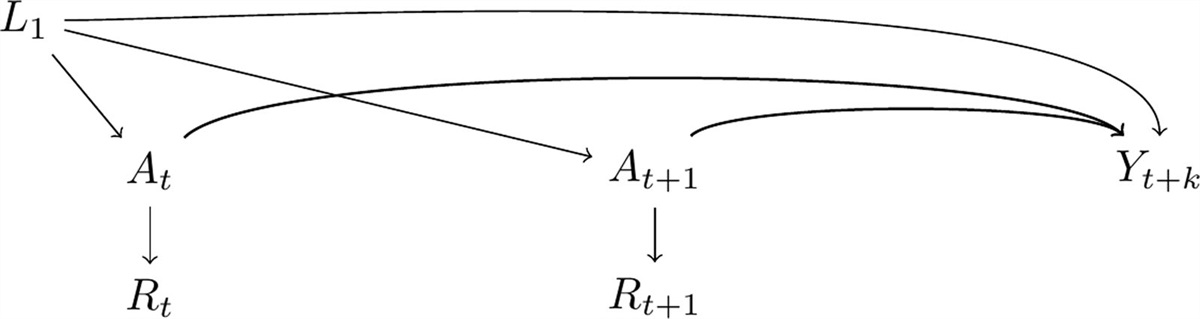
ASSUMPTION-FREE BOUNDS FOR TIME-VARYING TREATMENTS

The definition of consistency can also be generalized for time-varying treatments, though the notation requires alteration. Consider an exposure history through time kA¯i,k, an outcome Yi,k+1, and a vector of covariate histories L¯i,k for each individual at each time k∈[0,K]. Here, we use an overbar to represent history from time 0, that is,A¯k=(A0,A1,...,Ak). We denote counterfactual outcomes as Yi,k+1g, where g is some sustained treatment regime of interest that may be static or dynamic. Using this notation, we can define consistency for static and dynamic regimes formally as “for any strategy g, if Ai,kiscompatiblewithgk(A¯i,k−1,L¯i,k)) at each time k for each individual, then Yi,k+1g=Yi,k+1.”9 For expediency, we write Akiscompatiblewithgk(A¯k−1,L¯k)) as Ak=g(a,l) in later equations.

As with the time-fixed setting, we can bound counterfactual outcomes under a sustained treatment regime by imputing the best and worst possible outcomes for all individuals whose treatment history does not match the treatment regime we are interested in. For two arbitrary treatment regimes g and g′ in the set of all possible treatment regimes, the causal risk difference comparing the two is

E(Yk+1g)−E(Yk+1g′)=bylawoftotalprobabilityE(Yk+1g|A¯k=g(a,l))×P(A¯k=g(a,l))+E(Yk+1g|A¯k≠g(a,l))×P(A¯k≠g(a,l))−(E(Yk+1g′|A¯k=g′(a,l))×P(A¯k=g′(a,l))+E(Yk+1g′|A¯k≠g′(a,l))×P(A¯k≠g′(a,l)))=byconsistency

E(Yk+1|A¯k=g(a,l))×P(A¯k=g(a,l))+E(Yk+1g|A¯k≠g(a,l))×P(A¯k≠g(a,l))−(E(Yk+1|A¯k=g′(a,l))×P(A¯k=g′(a,l))+E(Yk+1g′|A¯k≠g′(a,l))×P(A¯k≠g′(a,l)))=bydefinitionforcategoricalvariablesE(Yk+1|A¯k=g(a,l))×P(A¯k=g(a,l))+E(Yk+1g|A¯k≠g(a,l))×(1−P(A¯k=g(a,l)))−(E(Y|A¯k=g′(a,l))×P(A¯k=g′(a,l))+E(Yk+1g′|A¯k≠g′(a,l))×(1−P(A¯k=g′(a,l)))).

Because E(Yk+1g) and E(Yk+1g′) are bounded between 0 and 1 for binary outcomes, we effectively impute these values for the unobserved counterfactual outcomes. Then the causal risk difference is bounded by:

E(Yk+1|A¯k=g(a,l))P(A¯k=g(a,l))+1∗(1−P(A¯k=g(a,l)))−(E(Yk+1|A¯k=g′(a,l))×P(A¯k=g′(a,l))+0∗(1−P(A¯k=g′(a,l))))≤E(Yk+1g−Yk+1g′)≤E(Yk+1|A¯k=g(a,l))×P(A¯k=g(a,l))+0∗(1−P(A¯k=g(a,l)))−(E(Yk+1|A¯k=g′(a,l))P(A¯k=g′(a,l))+1∗(1−P(A¯k=g′(a,l))))

which simplifies to

E(Yk+1|A¯k=g(a,l))×P(A¯k=g(a,l))+1−P(A¯k=g(a,l))−E(Y|A¯k=g′(a,l))×P(A¯k=g′(a,l))≤E(Yk+1g−Yk+1g′)≤E(Y|A¯k=g(a,l))×P(A¯k=g(a,l))−(E(Yk+1|A¯k=g′(a,l))×P(A¯k=g′(a,l))+1−P(A¯k=g′(a,l))).

Importantly, individuals who have not adhered to either treatment regime under study are not excluded from the analysis. Instead, because their outcome is unobserved for both regimes, their counterfactual outcomes under both regimes are imputed as the best or worst possible values. In addition to the causal risk difference, we can use this same approach to compute bounds on the counterfactual risk under each treatment strategy and the causal risk ratio (eTable 1; https://links.lww.com/EDE/C113, Figure). The quantities needed to compute these bounds can easily be derived from a Kaplan-Meier table.

FIGURE.: A, Bounds on the average causal effect of sequential monotherapy versus sequential dual non-SSRI therapy on risk of remission at 0, 1, 3, 6, and 9 months of follow-up among participants in the STAR*D trial who were initially assigned to citalopram and experienced treatment failure. B, Bounds on the counterfactual risk of remission under all three regimes of interest (sequential monotherapy, sequential dual non-SSRI therapy, sequential guidelines-based therapy) through follow-up in the same participants. All data were drawn from a secondary analysis of the STAR*D trial conducted by Szmulewicz et al.10

The width of the assumption-free bounds on the causal risk difference is therefore:

2−(P(A¯k=g(a,l)+P(A¯k=g′(a,l)).

Essentially, the width of the bounds on the risk difference is two (the width of the bounds on the risk difference without any data at all) minus the sum of the proportions of the eligible study population whose treatment history adheres to the two treatment regimes being compared (eMaterial; https://links.lww.com/EDE/C113). As previously stated, for a binary time-fixed treatment, the sum of the proportion of individuals who are adherent to one of the treatment regimes is equal to 1. However, for comparisons of mutually exclusive static regimes, such as “always treat” versus “never treat,” the width of the bound may be greater than 1 if the study population includes participants who do not adhere to either of the two regimes being compared (like participants who receive treatment for only some of the study period). For dynamic treatments, the width of the bounds may be smaller or larger than 1, depending on whether participants in the study have treatment histories that are compatible with both treatment regimes.

Consider a recent study aimed at estimating the average causal effect of sequential monotherapy versus sequential dual nonselective serotonin reuptake inhibitor therapy on depression remission among participants in the STAR*D trial who experienced treatment failure with citalopram10 (data partially reproduced in Table 1). At month 0, the treatment strategies for sequential monotherapy and sequential dual therapy are similar, with 698 of 971 participants compatible with sequential monotherapy, 492 compatible with sequential dual therapy, and 219 compatible with both. The width of the bounds on the average causal effect then reflects the 752 of 971 participants whose treatment history was compatible with only one regime (Table 2). In this example, we see the width of the bounds reduces to 2−(698971+492971)=0.77, less than 1 (Figure, eFigures 1 and 2; https://links.lww.com/EDE/C113). In contrast, at month 9, many participants’ treatment histories were incompatible with both regimes, and the width of the bounds is 1.47.

TABLE 1. - Data From an Analysis of the STAR*D Trial Among 971 Participants Who Experienced Treatment Failure on Citalopram, Comparing Sequential Monotherapy, Sequential Dual Nonselective Serotonin Reuptake Inhibitor Therapy, and Guidelines-based Sequential Therapy Treatment Arm Month Participants With Compatible Treatment Histories (n) Participants Who Experienced Remission (n) 1 0 698 0 1 1 692 29 1 3 355 114 1 6 283 173 1 9 280 180 2 0 492 0 2 1 469 24 2 3 268 112 2 6 234 154 2 9 231 162 3 0 525 0 3 1 513 19 3 3 263 97 3 6 222 147 3 9 220 152 This table shows the number of participants whose treatment strategies were compatible with each treatment strategy and the number of occurrences of remission in each arm at baseline and in months 1, 3, 6, and 9. Data are reproduced from Szmulewicz et al.10 A full description of the treatment strategies is available in the eMaterial; https://links.lww.com/EDE/C113.
TABLE 2. - Bounds on the Average Causal Effect of Regime 1 (Sequential Monotherapy) Versus Regime 2 (Sequential Dual Therapy) on Remission Among 971 Individuals in the STAR*D Trial Who Had Experienced Treatment on Citalopram Month Proportion of Participants Compatible With Regime 1 (n) Observed Mean Outcome Compatible With Regime 1 (n) Proportion of Participants Compatible With Regime 2 (n) Observed Mean Outcome Compatible With Regime 2 (n) ACE Lower Bound ACE Upper Bound 0 0.72 (698) 0 (0) 0.51 (492) 0 (0) 0.72 × 0 − (0.51 × 0 + 1 − 0.51) = −0.46 0.72 × 0 + 1 − 0.72 − 0.51 × 0 = 0.49 1 0.71 (692) 0.04 (29) 0.50 (481) 0.05 (24) 0.71 × 0.04 − (0.50 × 0.05 + 1 − 0.50) = −0.47 0.71 × 0.04 + 1 − 0.71 − 0.50 × 0.05 = 0.51 3 0.37 (355) 0.32 (114) 0.28 (268) 0.42 (112) 0.37 × 0.32 − (0.28 × 0.42 + 1 − 0.28) = −0.72 0.37 × 0.32 + 1 − 0.37 − 0.28 × 0.42 = 0.73 6 0.29 (283) 0.61 (173) 0.24 (234) 0.66 (154) 0.29 × 0.61 − (0.24 × 0.66 + 1 − 0.24) = −0.76 0.29 × 0.62 + 1 − 0.29 − 0.24 × 0.66 = 0.77 9 0.29 (280) 0.64 (180) 0.24 (231) 0.70 (162)