INTRODUCTION

In “Towards a clearer causal question underlying the association between cancer and dementia,” Rojas-Saunero et al.1 take a rare approach to discussing analytic choices and associated bias when interest is in a causal effect: they start with a story separate from the data in hand. Their story is about the causal effect of a Pin1-targeting drug on dementia risk. Embedded in their story are detailed, expert-communicated hypotheses about mechanisms by which Pin1 may act on cancer, dementia, and death. Pin1 is not measured in existing data sets available today to inform this effect. Further, no candidate for a drug with these properties has been identified or developed yet. However, Rojas-Saunero et al.1 clarify that the effects of unmeasured (hypothetical) treatments, such as a Pin1-targeting drug, implicitly motivate many investigators studying associations between cancer and dementia.

Leveraging Rojas-Saunero et al.’s example,1 I consider the benefits of a causal inference pedagogy and practice that leads with substantive stories. The arguments below are heavily inspired by Robins’s and Richardson’s work on extended causal graphical models and single world intervention graphs (SWIGs).2,3

CONSISTENCY DISENGAGED FROM STORIES

Epidemiology readers may be familiar with a long-running debate over the nature of the consistency condition in causal inference.4 One dominant position argues consistency is an assumption failing when there are “multiple versions of treatment,”5 rendering causal effects ill-defined.6,7 Another emphasizes an agnostic view to ill-defined effects, characterizing consistency as a definition that is a consequence of the investigator’s causal model.8 Formalized notions of “multiple versions of treatment”5 implicitly rely on a counterfactual causal model. Thus, the positions are seemingly best differentiated by whether or not one considers it possible to conduct valid and/or useful causal inference when premised on an ill-defined causal question.9–12 At the same time, there is apparent consensus in broadly characterizing consistency as a condition needed to link counterfactual variables to measured (observed) ones in the data in hand. Through Rojas-Saunero et al.’s example,1 we will see that this popularized characterization of consistency is a restricted case of a more general condition clarified only when we engage substantively with an investigator’s causal story.

Rojas-Saunero et al.1 consider different observed data scenarios for current studies of the cancer–dementia association and some covariate-adjusted approaches to analysis for each case. For exposition, I make some simplifications to their data structure, ignoring time-varying elements and presuming a population free of both cancer and dementia at baseline. Specifically, consider a study containing sample measurements (L,R,D,Y) from such a study population where L are baseline covariates (measured in the Rotterdam study1) and R,D and Y are indicators of incident cancer, death, and incident dementia, respectively, over follow-up. Rojas-Saunero et al.1 consider an inverse probability weighted (IPW) estimator that, given our simplifications and correctly specified weight models, may consistently estimate ψ~(r∗=1)−ψ~(r∗=0), where

ψ~(r∗)=∑lPr[Y=1|D=0,R=r∗,L=l]Pr[L=l].

Note, for simplicity and without meaningful loss of generality, here and throughout, all variables are considered discrete. On its own, (1) is nothing more than a function of the joint distribution of measured variables in this study. It is a reduced case of Robins’s g-formula13 and can be estimated using different statistical methods under different assumptions on this distribution.14–16 Such methods are popularly termed causal inference methods. A widely adopted pedagogical premise for this causal classification, and the foundation for the consistency debate referenced above, is the following: For all individuals, define Yr∗,d=0 as their counterfactual (potential) outcome had R been forced to fixed value r∗ and D forced to fixed value d=0. Suppose two assumptions hold for both r∗=1 and r∗=0: exchangeability

Yr∗,d=0∐D|R=r∗,L=landYr∗,d=0∐R|L=l

and consistency

IfR=r∗andD=0thenY=Yr∗,d=0.

Then, provided a positivity condition also holds ensuring the observed data function (1) is defined for r∗=1 and r* = 0,17 we can prove the average causal effect of ensuring, versus preventing, cancer on risk of dementia over follow-up, had death been also eliminated, or Pr[Yr∗=1,d=0=1]−Pr[Yr∗=0,d=0=1], equals the observed data function ψ~(r∗=1)−ψ~(r∗=0) because Pr[Yr∗,d=0=1]=ψ~(r∗).14,18

Given my own lack of expertise in this subject matter, the information considered in this section alone is insufficient to communicate the investigator’s intent. This information was limited to a description of who and what was measured in the current study and the nature of statistical code run on a data set. By this, I would classify the counterfactual quantity Pr[Yr∗=1,d=0=1]−Pr[Yr∗=0,d=0=1] as ill-defined because no causal story is provided to clarify its meaning or even to confirm that this quantity correctly formalizes what the investigator wants to know. We solve this by engaging with Rojas-Saunero et al.’s motivating causal story.1 This story confirms that, in this case, an effect indexed by an intervention r∗,d=0 does not formalize what is of interest. Engaging with the details of this story is necessary for correctly formalizing what is of interest and, in turn, correctly reasoning about the nature of possible bias in statistical methods constructed for (1), whether there are better alternatives for leveraging existing data today, what those alternatives are, and how to improve future study designs.

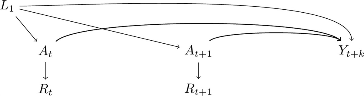
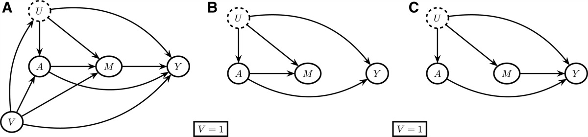
CONSISTENCY LED BY STORIES

The causal directed acyclic graph (DAG)19 in Figure 1 is similar to those presented by Rojas-Saunero et al.1 but with time-varying elements removed. This depicts at least one crucial component of their story missing from the formalization above: unmeasured Pin1 (A). Figure 2A extends Figure 1 further to add a node Z representing the unmeasured treatment referenced in their story: an indicator of receiving a drug targeting Pin1. I will consider Z a random variable, reflecting a setting where the drug exists and is available: some individuals receive it (Z=1), others do not (Z=0). We consider Z unmeasured because investigators do not have a measure of it in their data set. Foundations for a logically similar, slightly more technical, thought process where the drug does not yet exist (such that Z=0 for all individuals) can be found in the recent literature on separable effects,2,21–25 also considered below. Figure 2 also assumes Z shares no common causes with other variables relevant to the story (depicted on the DAG) as in a study where Z is physically randomized but also in an observational study stratified on all common causes of Z and other nodes.

FIGURE 1.: A causal directed acyclic graph similar to those presented in Rojas-Saunero et al.1 simplified for exposition to remove time-varying elements. This explicitly depicts a key part of their communicated story, Pin1 (

A

), that would never be understood knowing only that a statistical method widely classified as a “causal inference method” was implemented using only observations of

L,R,D,Y

, with

R

(an indicator of incident cancer) playing the “typical role” in statistical code of “treatment,”20 and

D

(an indicator of death) the “typical role” of “censoring.”18FIGURE 2.: The graph in (A) extends the causal directed acyclic graph in Figure 1 further to include

Z

, an indicator of receiving a drug targeting Pin1 expression, the treatment in their story. The single arrow out of

Z

into

A

implicitly communicates the assumption that changing

Z

can only affect cancer and dementia via

A

. The graph in (B) is a Single World Intervention Graph3 that, under a consistency assumption with respect to counterfactual outcome

Yz

, is an even more explicit representation of the counterfactual causal model underlying (A). This counterfactual is defined relative to this model. The graph in (B) is a node-splitting transformation of the graph in (A) where only the treatment is split. Variables in (B) indexed by

z

are the counterfactual natural values of variables had this intervention been implemented.3 Their capitalization reflects the assumption that intervention

z

would not deterministically control their values to a fixed level for all individuals.

The SWIG3 in Figure 2B is an intervention-specific transformation of Figure 2A that explicitly depicts counterfactuals defining an effect more closely aligned with Rojas-Saunero et al.’s story:1 an average causal effect of Z=1 (versus Z=0) on Y:

Pr[Yz=1=1]−Pr[Yz=0=1].

This is defined relative to the causal model in Figure 2B, clarifying that Yz is the dementia status an individual would have had if Z were set to fixed value z and all variables affected by intervention take their counterfactual natural values under z.3 These are capitalized to signal they may vary across individuals all receiving treatment z (a realistic characterization of drugs targeting biological processes, e.g. blood pressure, cholesterol). Figure 2 also encodes a mechanistic assumption that Z affects R,D and Y only via A (Pin1). We will return to the implications of assumptions on treatment mechanism for the target effect itself below. Given the causal model in Figure 2, the following alternative exchangeability condition

Yz∐Z

can be read directly from Figure 2B.3 An alternative consistency condition

IfZ=zthenA=Az,R=Rz,D=Dz,Y=Yz

relates Figures 2A and 2B3. This consistency condition is distinct from that in (3) in two important ways. First, it references a different counterfactual outcome that would never have been formalized without engaging with a more detailed story. Second, it is a condition that links counterfactual to factual, but possibly unobserved, variables. Given these alternative exchangeability and consistency conditions, we can equate (4) to ψ(z=1)−ψ(z=0), where

ψ(z)=Pr[Y=1|Z=z]

provided a positivity condition also holds ensuring this factual data function is defined. This is a factual (rather than counterfactual) data function, but it is not observed because Z is unmeasured. We cannot unbiasedly estimate it without additional assumptions restricting the joint distribution of the factual random variables in our causal story. Such assumptions are generally at odds with dependencies allowed under the model in Figure 2. However, this challenge to causal inference is not the result of an ill-defined question. It is the result of limitations in the data in this particular study. Our reasoning here also provides a more precise understanding of structural/causal bias than that communicated only via a causal DAG26 that does not depict counterfactuals. For the target (4) defined by the causal model in Figure 2, the structural bias associated with an IPW (or other) statistic constructed for (1) can be more transparently understood as whether and the degree to which

[ψ~(r∗=1)−ψ~(r∗=0)]−[ψ(z=1)−ψ(z=0)]≠0

In this alternative exposition, we never invoked the consistency assumption (3) to reason about bias. In turn, this alternative story-led thought process has real implications for improved scientific practice. This includes providing a correctly guided foundation for describing study limitations in a discussion, development of sensitivity analysis and/or partial identification bounds, and improving data collection in future studies. If the data in hand (L,R,D,Y) is the best available today to inform this question, our thought process led by a story can also clarify how to better leverage it.

For example, the independencies encoded in Figure 2 allow us to rewrite (7) as

ψ(z)=∑a,r,lPr[Y=1|D=0,A=a,L=l]Pr[D=0|R=r,L=l]×

Pr[R=r|A=a,L=l]Pr[A=a|Z=z,L=l]Pr[L=l]

Consider an alternative observed data function

ψ~(z)=∑r,lPr[Y=1|D=0,R=r,L=l]Pr[D=0|R=r,L=l]×

Prz[R=r|L=l]Pr[L=l],

where we will understand Prz⁡[R=r|L=l] as a (possibly wrong) guess at the distribution of R given L=l, marginal over A, had the intervention z been implemented. ψ~(z) is a generalized version13,27 of the g-formula ψ~(r∗) in (1) we considered absent any story. The two coincide when no deaths actually occur in the population (not the case) and we select Prz⁡[R=r|L=l]=1forr=r∗and0forr≠r∗, a guess that receiving Z=z ensures cancer status r∗ in everyone deterministically (incompatible with our story). Therefore, a statistic constructed for ψ~(z), allowing that deaths occur and allowing a more substantively informed guess at this intervention distribution, seems a more reasonable way to leverage existing data (L,R,D,Y). If we perfectly guessed

Prz[R=r|L=l]=∑aPr[R=r|A=a,L=l]Pr[A=a|Z=z,L=l],

then ψ(z) and ψ~(z) differ by the terms Pr[Y=1|D=0,A=a,L=l] and Pr[Y=1|D=0,R=r,L=l], respectively. By this difference, and that our guess will never be perfect, such a statistic will generally be biased. However, it might reasonably be less biased than the original statistic for ψ~(r∗) considered absent any story. “Less biased” here formally means:

abs([ψ~(r∗=1)−ψ~(r∗=0)]−[ψ(z=1)−ψ(z=0)])>

abs([ψ~(z=1)−ψ~(z=0)]−[ψ(z=1)−ψ(z=0)])

If z would decrease Pin1 expression, reducing cancer incidence, then one guess at Prz⁡[R=1|L=l] could be a specified downward shift in the observed Pr[R=1|L=l]. IPW and nonparametric double/debiased28 statistics for this “incremental propensity score”29 specification of (10) are developed and practically implemented.29–32 This literature has only explicitly justified these methods for stochastic interventions, naively in this case, on R. This story clarifies an alternative motivation for such methods by deterministic interventions on unmeasured treatments, requiring alternative causal reasoning as just illustrated. Related arguments are formalized elsewhere.3,33,34

TRIALS DO NOT ESCAPE STORIES

Suppose now we did conduct a study where Z is randomized and measured along with (A,R,D,Y). This trial constitutes a “Target Trial” when our question is Pr[Yz=1=1]−Pr[Yz=0=1].35,36 However, we still have not considered an important aspect of Rojas-Saunero et al.’s story:1 death. Rojas-Saunero et al.1 acknowledge effects under “elimination of death” are not of interest, but rather effects that isolate separate mechanisms by which Pin1 operates on dementia and cancer, in the real world, where deaths unfortunately occur. The effect Pr[Yz=1=1]−Pr[Yz=0=1], defined by the model in Figure 2, does not address this question because, with A overall Pin1, this is a total effect18,37 possibly capturing hypothesized “opposing” Pin1 mechanisms.1 Thus, this trial is actually not the “Target Trial.”

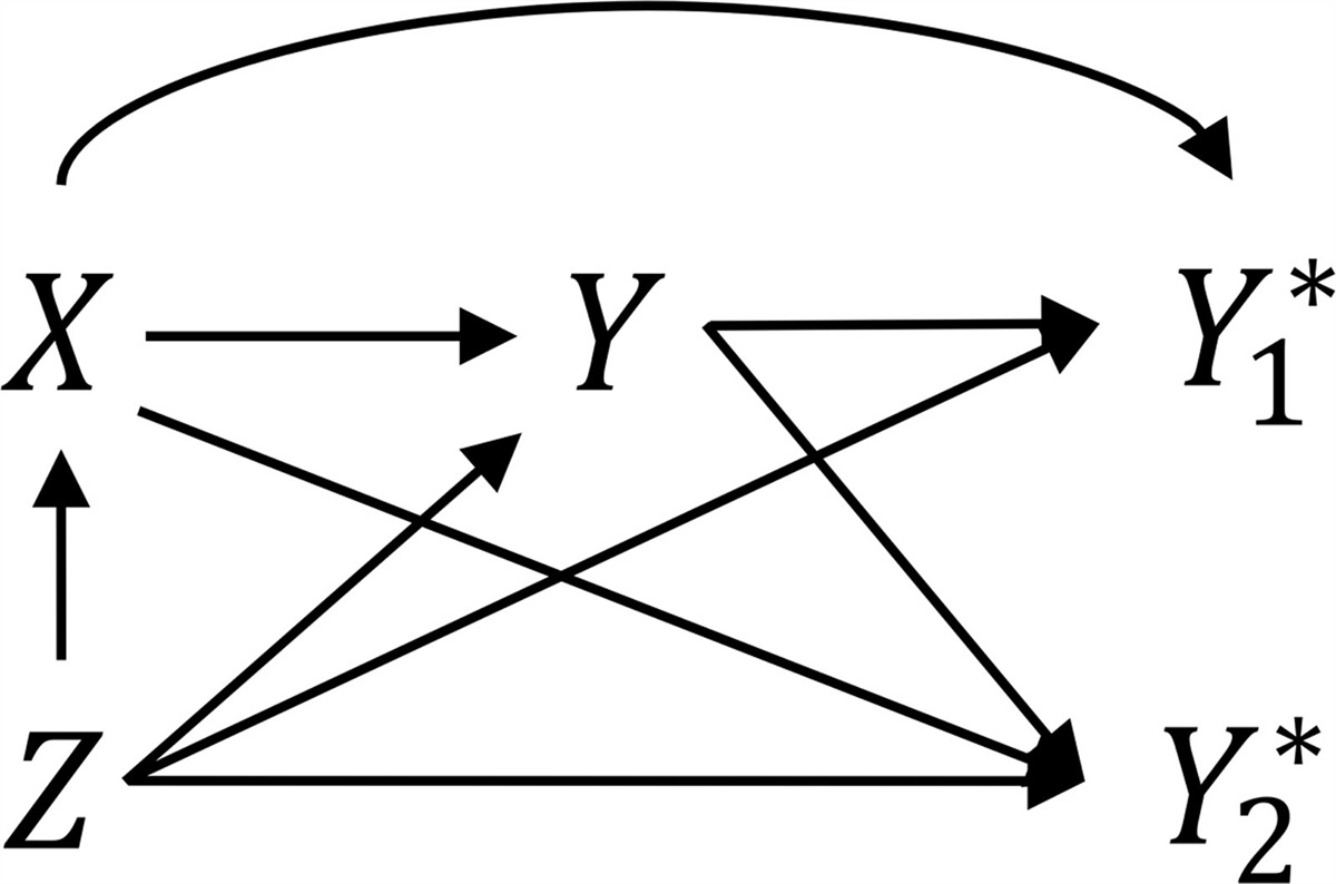
Figure 3 extends the story to align with this goal, separately depicting hypothesized Pin1 expression affecting the brain (AY) and cancer development (AR). ZY and ZR might represent modifications of Z to target Pin1 in these specific areas: ZY targeting increases in AY (hypothesized to prevent dementia) and ZR