Most epidemiologic evidence regarding the health impacts of long-term exposures to air pollution—or other environmental exposures—has been obtained through observational cohort studies. However, spurious associations, sometimes counterintuitive and labeled as paradoxes, may commonly occur in such observational settings and be underreported in the published literature. These spurious associations can be due to a discrepancy between the study population and the target population.1(chap14) This lack of representativeness or selection bias has been dismissed by some authors,2 but it has the potential to generate misleading associations.3 Differential participation, which occurs frequently in observational cohorts, especially those studying the etiologic effects of long-term environmental exposures, is one likely cause of the discrepancy between the study and target populations.

Differential participation arises from non-participation when subjects in the target population (1) opt not to participate (i.e., nonresponse) or (2) have the outcome of interest before the start of follow-up and thus are not eligible, leading to these outcomes being excluded from the cohort (i.e., left truncation).4,5 Since most cohorts only enroll subjects free of the outcome of interest (by design) and healthy enough to participate (in practice), the outcome is generally associated with the probability of participation directly or via shared risk factors. If the magnitude of nonparticipation does not differ by the exposure of interest (i.e., nondifferential participation), analytical methods such as Cox proportional hazards models can account for it by only including person-times observed in the analysis and will estimate unbiased associations.6 However, in real-life settings, participation is unlikely to be independent of long-term environmental exposures, and this can lead to misleading associations due to conditioning on a common effect of exposure and outcome (i.e., collider stratification bias with participation as the collider).7

Selection bias caused by differential participation has been described in observational cohort studies of nonenvironmental exposures and is sometimes referred to as left truncation,8,9 left informative censoring,10,11 non-representative,12 nonresponse bias,5,13,14 healthy worker bias,4 survival bias,15 live-birth bias,16 index event bias,17 or simply as collider bias and selection bias.18–21 A well-known example is the paradox in which smoking (i.e., exposure) appears to confer a counterintuitive protective effect against preeclampsia in a pregnancy cohort.22,23 This paradox can be explained by collider bias due to differential participation in the target population of all pregnancies—only subjects not experiencing early pregnancy loss were enrolled into the study population and followed for preeclampsia, while early pregnancy loss (i.e., a collider) is both affected by smoking and abnormal placentation, a shared risk factor with preeclampsia. In other words, among cohort participants or pregnant women not experiencing early pregnancy loss, smokers were less likely to have abnormal placentation and subsequent preeclampsia, which leads to a counterintuitive protective effect of smoking on preeclampsia.

Cohorts studying etiologic effects of long-term environmental exposures are especially susceptible to experiencing counterintuitive associations caused by differential participation because environmental exposures are generally prevalent in the target population long before the cohort enrollment and could impact participation via frailty or related geographic factors. Moreover, the expected effects of most environmental exposures are relatively small, making it easier for a reversed association to occur even in the presence of a small bias. However, the literature on differential participation in observational cohorts of environmental epidemiology is limited. Existing publications have mostly focused on specific subpopulations such as birth cohorts and occupational cohorts, in which the bias is caused by a necessary restriction of analysis to live births,16,24 pregnancies without early loss,22,25 or existing employees.4 Yet, using cohorts of the general population may similarly yield counterintuitive associations due to differential participation, but such issues have not been discussed to date.

In this article, we provide an in-depth discussion of differential participation in observational cohorts of the general population and how it might cause spurious or even counterintuitive associations in environmental health research. We also discuss the washout method as one potential analytical solution to account for such bias without the need for additional data on nonparticipants or shared risk factors between participation and outcome. Specifically, we first discuss key points to consider in evaluating and accounting for differential participation. We also use causal graphs to describe two possible bias mechanisms caused by differential participation (geographic factor-driven and frailty-driven). Next, we demonstrate the existence of a counterintuitive association in a survey-based national observational cohort studying fine particulate matter (PM2.5) and mortality and apply the washout method in this real-life example. Last, we conduct simple simulations to mimic the counterintuitive associations observed in the real-life example and demonstrate the efficacy of the washout analysis.

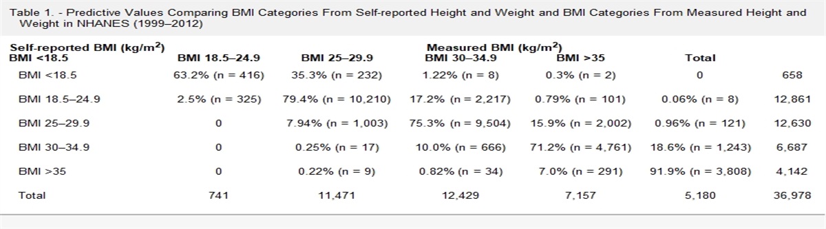
METHODS How to Evaluate and Account for Differential Participation

We include a list of key points to consider in evaluating and accounting for differential participation in Table 1. To evaluate whether selection bias exists in an observational cohort, we need to specify the target population, which should be based on the research question of interest (Question 1 of Table 1). In this article, we assume that the target population is a population free of the outcome at cohort initiation. Second, we need to assess whether differential participation may exist between the study cohort and the target population based on our substantive knowledge of relationships among exposure, outcome, and potential reasons for nonparticipation (Question 2 of Table 1). Below, we describe two distinct mechanisms through which such differential participation bias can occur and cause spurious exposure-outcome associations in etiological studies of environmental exposures (Evaluation 2.1 of Table 1). Both mechanisms depend on the fact that only those who survived until the start of follow-up and were healthy enough before enrollment can enroll in the observational cohort studying long-term environmental exposures.

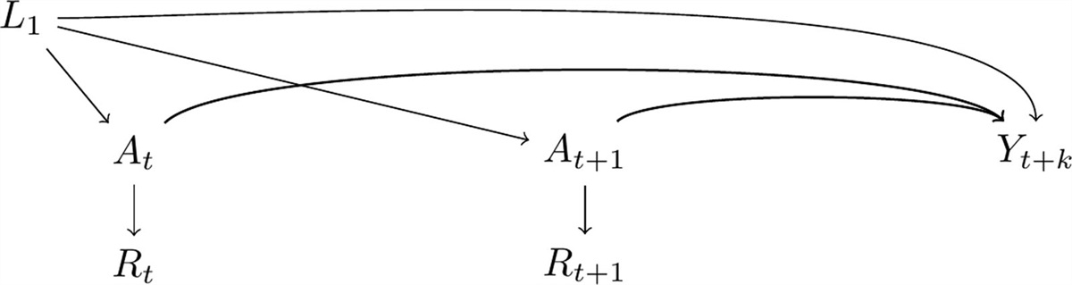
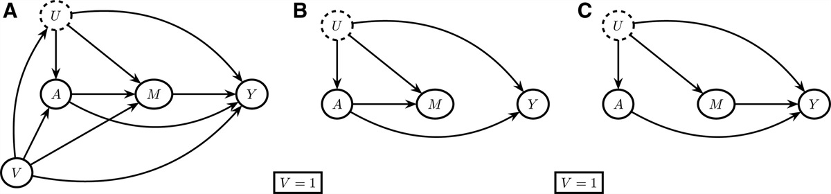
TABLE 1. - Key Points to Consider in Evaluating and Accounting for Differential Participation Question Exploratory Analyses/Evaluations 1. What is the target population? Specified based on the research question 2. Is there differential participation (discrepancy between the cohort and the target population)? 2.1. Draw causal graphs based on subject-matter knowledge and evaluate whether participation creates a backdoor path based on causal graphs.
2.2. Evaluate the extent to which the distributions of exposure and outcome in the study cohort deviate from their expected distributions in the target population (can suggest the presence of differential participation but cannot verify the lack of differential participation).
2.3. Calculate time-varying effect estimates such as adjusted survival curves and evaluate whether any observed differences in effect estimates over time are consistent with subject-matter knowledge. 3. How to account for bias due to differential participation in effect estimates? 3.1. With additional data from nonparticipants, use inverse probability weighting on participation (or selection) models.
3.2. With additional data on all risk factors shared by participation and outcome, control for them using any method.
3.3. Without additional data, conduct a washout method that drops the first few years of follow-up. A naïve analysis including all follow-up years might be conducted first to help identify the years to be dropped.

The first example is a frailty-driven mechanism (Figure 1A). The prebaseline health status would determine the probability of participation in the study. Since many environmental exposures are prevalent in the target population long before the start of follow-up and are affecting the probability of surviving or being outcome-free, we would expect to see differential participation bias in such cohorts as long as the environmental exposure has a causal effect on the prebaseline health status (e.g., alive, outcome-free, and healthy enough to participate) and there exists an unmeasured shared risk factor (e.g., unobserved baseline frailty such as respiratory infection) between the prebaseline health status and the probability of having the outcome during follow-up.26 For example, when investigating the effect of air pollution on mortality in a cohort of recruited participants, those who are too sick at baseline will decline to participate in the study. Assuming air pollution, in combination with other causes of illness, makes people unhealthy to participate in the study, an inverse correlation will emerge between air pollution and mortality through other causes of illness among the participants. That is, among those healthy enough to participate, individuals previously exposed to worse air pollution are less likely to have another unrelated health risk factor such as respiratory infection, and the lack of such risk factor would decrease their chances of mortality.27(p100) The bias arising from selecting participants alive and outcome-free differs from the bias stemming from selecting participants healthy enough to participate. One could argue that a target population is defined as those free of the outcome at the time of enrollment, and the susceptible population is stable in the target population. Subsequently, one could assert that no differential participation exists in the study population. However, many cohorts also require voluntarily active participation from the subjects, such as completing a questionnaire or attending a medical appointment, which could lead to a stronger connection between exposure and participation through being healthy enough to actively participate at the time of enrollment than simply being outcome-free.28

FIGURE 1.:

Causal graphs for two mechanisms in which differential participation could cause a spurious association between environmental exposure and adverse health outcomes. Bias still exists even if we remove the arrows between exposure and outcome, assuming no direct effect. A, frailty-driven mechanism. B, Geographic factor-driven mechanism.

The second example is a geographic factor-driven mechanism (Figure 1B). Even if the environmental exposure does not affect the prebaseline health status of potential participants, participation could be connected to exposure via their spatial associations with geographical regions. Environmental exposures generally demonstrated spatial heterogeneity across geographical regions. Such geographical regions could be related to participation due to a variety of technical and social reasons. Particularly, cohorts based on existing datasets that were collected for purposes other than studying the etiologic effect of environmental exposure are being increasingly used in studies of environmental exposures, in which a sampling scheme intrinsically involving geographic factors is likely. For example, a survey targeted to study the general population might sample more participants from the urban area for operational reasons, while urbanicity is associated with higher environmental exposures such as air pollution. Such sampling schemes can lead to an open backdoor path between exposure and outcome through participation. This geographic factor-driven bias mechanism would exist even when the environmental exposure of interest is new instead of prevalent.

Although presented separately here, both mechanisms can co-exist in the same cohort. The association between exposure and outcome observed in cohorts affected by either or both mechanisms could be attenuated or even reversed from the true effect in the target population. Empirical evidence of disparity in exposure and outcome distributions between participants and nonparticipants or between the study population and the target population might suggest differential participation (Evaluation 2.2 of Table 1). However, the lack of disparity in such distributions does not rule out the possibility of differential participation and spurious exposure-outcome association.5,29 As a complementary step, estimating time-varying effect estimates like adjusted survival curves could also aid the identification of differential participation as it allows the effect to vary over time, and counterintuitive effects at the beginning of follow-up might suggest differential participation (Evaluation 2.3 of Table 1).

Although differential participation is ideally prevented at the stage of study design, such induced bias could also be controlled via statistical methods in the analytical stage. For example, if we had extra information on those not participating, we could use inverse probability weighting of participation in our analysis to create a pseudo population not affected by differential participation,15,30 or use selection models to account for informative missingness (Analysis 3.1 of Table 1).11 If we had information on all risk factors shared by prebaseline health status and outcome, we could also control for them in epidemiologic models to eliminate or mitigate the bias (Analysis 3.2 of Table 1).31 However, the above correction methods are infeasible if the required additional data were not collected before the analytical phase, which is very likely. In such settings, where this bias cannot be addressed by considering additional measured covariates, a simple washout method (by removing data from the first few years of follow-up) has been proposed as a possible solution (Analysis 3.3 of Table 1).32,33 Some studies, in nonenvironmental settings, have employed a washout analytical method so that the impact of differential participation would decrease as people with high baseline frailty either died or recovered during the washout period and the remaining study population could better approximate the target population.34–36 Empirically, the period to be removed could be determined by identifying the elbow or turning point in the adjusted survival curves of the naïve analysis (including all follow-up years), before which the differential participation bias was still strong.32 Below, we demonstrate the effect of differential participation bias in a real-life example, employ the washout analytical method to account for this bias, and conduct a simulation study to demonstrate the efficacy of this method.

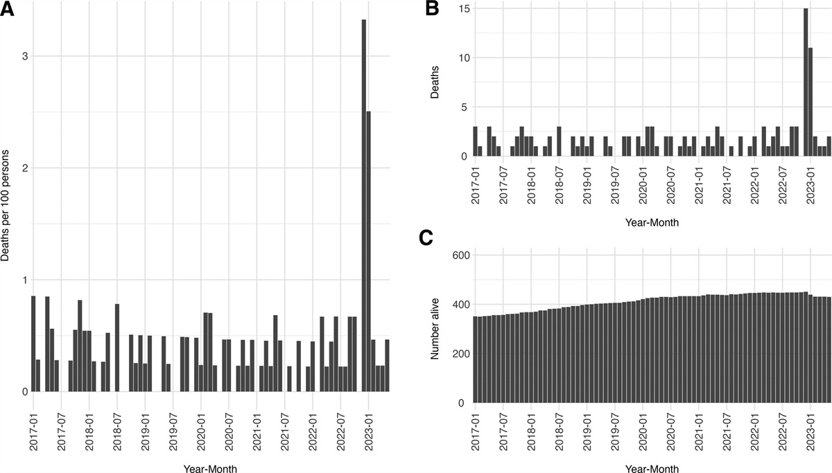
Real-life Example: The Canadian Community Health Survey

With a retrospective cohort of respondents to the Canadian Community Health Survey (CCHS), we demonstrate the emergence of counterintuitive associations and the effect of the washout method in accounting for bias. Employing the parametric g-computation demonstrated in Chen et al.37 2023, we aim to evaluate the effectiveness of hypothetical intervention strategies targeting long-term exposure to PM2.5 in this real-life example through the comparison of adjusted survival curves with and without the intervention. CCHS is a cross-sectional survey of the general Canadian population for multiple enrolling cycles.38 For illustration, we used data from the 2000/2001 enrolling cycle. We obtained data on the participants’ vital statistics, annual exposure to PM2.5, and other time-varying and time-fixed covariates between the survey date (cohort inception) and 31 December 2014 (the end of follow-up) via linkage to administrative datasets and previously estimated exposure surfaces. Several published articles studying environmental exposures used multiple enrollment cycles from this cohort and reported further details.39,40 Here we list a few relevant aspects of the cohort (Evaluation 2.1 in Table 1). First, although aimed to study the general population, participation in the CCHS was voluntary and a complete response required participation in an in-person or telephone interview,38 which inherently restricted the participants to be healthier than the general population and might have caused frailty-driven differential participation (Figure 1A). Second, this cohort used health regions to aid sampling and over-sampled rural communities,39 which might cause geographic factor-driven differential participation (Figure 1B).

To explore whether differential participation exists, we plotted age group-specific 4-year cumulative mortality rates over time (Evaluation 2.2 in Table 1). To estimate the adjusted survival curve with and without intervention, we conducted a naïve analysis without considering potential differential participation using 10 years of follow-up data from 2000/2001 to 2010 (Evaluation 2.3 in Table 1). To save computation time, we did not use all 14 years of follow-up in naïve analysis. Specifically, we conducted a parametric g-computation analysis to evaluate the potential health benefits of a hypothetical intervention that reduces participants’ long-term exposure to PM2.5 to 5 μg/m3 if they were exposed to PM2.5 higher than 5 μg/m3, compared to having no intervention. We included a 3-year moving average of PM2.5, indicators for the year, interaction terms between year and PM2.5, rurality, a spline function of age with five knots, and other potential confounders in the pooled logistic model for outcome as part of the parametric g-computation. We included urbanicity as a covariate in the outcome model, and therefore the bias pathway shown in Figure 1B is likely blocked (assuming rurality is the only geographic factor affecting participation). We estimated the 95% confidence intervals of differences in survival probabilities between interventions using standard errors from 200 bootstrap iterations. More details on this analysis were discussed elsewhere.37

Next, as an approach to account for differential participation, we applied the washout method by removing observations in the first 4 years of follow-up by delaying the cohort entry until 2005, with a total of 10 years of follow-up data until 2014, followed by repeating the parametric g-computation analysis (Analysis 3.3 in Table 1). We incorporated four more years of follow-up than those utilized in the naïve analysis so that the length of follow-up would be comparable. We decided to delay the cohort entry until 2005 because the difference in survival probability reached the inflection point in the fifth year in the naïve analysis (Figure 2A), suggesting that the bias caused by differential selection was weakened from that time point onwards. In addition, we excluded those older than 79 in 2005 in the washout analysis to ensure that all participants would be followed for up to 10 years or until death because the original administrative dataset censored individuals after age 89.

FIGURE 2.:

Difference in survival probability (5 μg/m3 threshold intervention minus no intervention) over time estimated with parametric g-computation in the CCHS cohort. A, naïve analysis in using 10 years of follow-up. B. Washout analysis where the first 4 or 5 years of follow-up are dropped. Shadowed bands are 95% confidence intervals estimated with bootstrapping.

Last, to facilitate comparison with traditional survival analysis methods, we repeated the naïve and washout analyses using a Cox proportional hazards model and an Aalen additive hazard model with 3, 5, and 10 years of follow-up. Like previous studies using traditional survival analysis methods, we assumed a constant association between PM2.5 and mortality and included the same set of confounders as those used in the outcome model of parametric g-computation other than indicators for the year and interaction terms between year and PM2.5. All analyses of the CCHS cohort were carried out in R version 4.0.541 and relevant codes for g-computation can be found at: https://github.com/suthlam/cchs_g_computation.git. The Health Canada-Public Health Agency of Canada Research Ethics Board approved the study.

Simulation Scenarios

For illustrative purposes and to demonstrate that the two hypothesized bias mechanisms discussed above could plausibly attenuate or even reverse the true effect, we conducted simulations for each mechanism separately based on causal graphs in eFigure 1; https://links.lww.com/EDE/C103. The underlying structures of bias are the same as shown in Figure 1 except that we added the direct effect from exposure to the outcome and updated the label of the knot to mimic the CCHS example for easier interpretation.

We generated time-to-event data using structural equations of additive hazards with modified simulation codes from Strohmaier et al. 2015.42 To mimic the real world, we used coefficients based on statistics and effect estimates from the CCHS cohort (e.g., 0.0002 increase in hazard rate per 1 μg/m3 increase in PM2.5 for the association between PM2.5 and mortality). For simplicity and didactic purposes, we used time-fixed exposure and assumed no direct effect from baseline frailty (frailty-driven mechanism) or prebaseline health status (geographic factor-driven mechanism) on death after 3 years of follow-up. We also assumed no unmeasured confounding between residential PM2.5 and mortality. The simulation involved three steps: (1), we simulated a full cohort of 100,000 individuals with 10 years of follow-up and no differential participation; (2) we created an observed cohort by only including 70% of individuals with the highest probability of participating at baseline, which is affected by a geographic factor (geographic factor-driven mechanism only) and the prebaseline health status (both mechanisms) separately; and (3) we iterated each simulation 100 times. Specific coefficients and distributions used in the simulation are included in eAppendix 1; https://links.lww.com/EDE/C103.

To estimate the association between PM2.5 and death, we repeated the same analyses for the simulated full cohort (representing the target population) and observed cohort (representing the analytical cohort) separately as we did for the CCHS cohort: g-computation, Aalen model, and Cox model with and without applying the washout method. The maximum length of follow-up year is 10 in naïve analysis and seven in washout analysis. Details are included in eAppendix 2; https://links.lww.com/EDE/C103. Aside from visually comparing summaries of effect estimates from the full and observed cohorts, we also calculated absolute bias as the difference between effect estimates in the observed cohort and the corresponding full cohort before summarizing the bias across iterations. This comparison used estimates from the full cohort as the target parameters and reduced the influence of random errors generated by the data simulation process. We report absolute biases from the Aalen model and relative biases from the Cox model (percentage difference in hazard ratios between the observed and the full cohort). 95% simulation intervals (SIs) were calculated using the Wald standard error of estimates from the 100 iterations. All simulations and analyses were carried out in R 4.1.0 and relevant codes can be found at: https://github.com/suthlam/differential_participation_simulation.git.

RESULTS

The naïve analysis of the CCHS cohort included a final cohort of 65,470 individuals. Using parametric g-computation, we found negative values for the difference in annual probabilities of survival (with the 5 μg/m3 threshold intervention minus without intervention) during most years of follow-up (Figure 2A), suggesting a worse survival probability in the study population after reducing the level of ambient PM2.5. This finding is contrary to subject-matter knowledge about the harmful effect of chronic exposure to PM2.5 on mortality.43 Additionally, we observed low cumulative mortality rates in the first few years of follow-up across all age groups (eFigure 2; https://links.lww.com/EDE/C103). Results from the Aalen model and the Cox model were consistent with those from the g-computation, with null or negative associations between residential PM2.5 and mortality across all follow-up periods (Table 2, eFigure 3A and C; https://links.lww.com/EDE/C103).

TABLE 2. - Effect Estimates When Differential Participation Exists With and Without Applying the Washout Method in Analysis by Cohort, Model, and Length of Follow-up Time Cohort Analysis Length of Follow-up Time Hazard Difference Per Unit Change in PM2.5 per 1000 Persons
(95% CI for CCHS, 95% SI for Simulated Cohorts)
(Aalen model) Hazard Ratio Per Unit Change in PM2.5 (95% CI for CCHS, 95% SI for Simulated Cohorts)
(Cox Model) Full Cohort Observed Cohort Full Cohort Observed Cohort CCHS Naïve 3-year NA 0.03 (−0.15, 0.22) NA 0.99 (0.96, 1.03) 5-year −0.18 (−0.36, −0.01) 0.98 (0.96, 1.00) 10-year −0.13 (−0.29, 0.02) 0.99 (0.98, 1.01) Washout 3-year 0.40 (0.10, 0.70) 0.99 (0.96, 1.03) 5-year 0.63 (0.38, 0.87) 1.01 (0.98, 1.04) 10-yeara 0.38 (0.19, 0.58) 1.01 (0.99, 1.03) Frailty-driven simulation Naïve 3-year 0.12 (−0.06, 0.29) −0.05 (−0.26, 0.17) 1.02 (1.00, 1.04) 0.99 (0.97, 1.02) 5-year 0.15 (0.03, 0.27) 0.01 (−0.16, 0.17) 1.02 (1.01, 1.04) 1.00 (0.98, 1.03) 10-year 0.18 (0.09, 0.27) 0.11 (−0.01, 0.22) 1.02 (1.01, 1.04) 1.02 (1.00, 1.03) Washout 3-year 0.13 (−0.04, 0.30) 0.14 (−0.07, 0.35) 1.03 (1.00, 1.05) 1.03 (0.99, 1.06) 5-year 0.16 (0.02, 0.29) 0.16 (−0.02, 0.35) 1.03 (1.01, 1.04) 1.03 (1.00, 1.05) 7-yearb 0.17 (0.07, 0.28) 0.18 (0.03, 0.32) 1.03 (1.01, 1.04) 1.03 (1.01, 1.05) Geographic factor-driven simulation Naïve 3-year 0.12 (−0.01, 0.25) −0.01 (−0.16, 0.13) 1.02 (1.01, 1.04) 1.00 (0.98, 1.02) 5-year 0.16 (0.07, 0.25) 0.03 (−0.08, 0.15) 1.02 (1.01, 1.04) 1.01 (1.00, 1.02) 10-year 0.18 (0.11, 0.25) 0.12 (0.04, 0.2) 1.03 (1.02, 1.03) 1.02 (1.01, 1.03) Washout 3-year 0.14 (0.02, 0.26) 0.13 (−0.01, 0.27) 1.03 (1.01, 1.05) 1.03 (1.01, 1.05) 5-year 0.16 (0.06, 0.27) 0.17 (0.05, 0.28) 1.03 (1.01, 1.04) 1.03 (1.01, 1.05) 7-yearb 0.17 (0.09, 0.26) 0.18 (0.07, 0.29) 1.03 (1.02, 1.04) 1.03 (1.01, 1.04)

aIn the real-life example of CCHS, we have 14 years of follow-up time thus it is possible to have 10 years of follow-up time after dropping the first 4 or 5 years of follow-up in the washout analyses.

bIn the simulation, we created a cohort with 10 years of follow-up time thus we only have 7 years of follow-up time after dropping the first 3 years of follow-up in the washout analyses.

After applying the washout method to the CCHS cohort, the cohort size was reduced to 62,365. The estimated differences in annual probabilities of survival were positive during 10 years of follow-up after applying washout analysis, suggesting a beneficial effect of PM2.5 reduction on mortality (Figure 2B). We also observed positive associations for all follow-up periods in the Aalen model (Table 2, eFigure 3A; https://links.lww.com/EDE/C103), while the associations were null in the Cox model (Table 2, eFigure 3C; https://links.lww.com/EDE/C103).

Using simulations with the frailty-driven and geographic factor-driven mechanisms, we successfully mimicked the patterns of estimates observed in the naïve analysis of the CCHS cohort in the observed cohort simulated. Like g-computation results from the CCHS cohort, we observed negative differences in survival probability comparing 5 μg/m3 threshold intervention to no intervention under both bias mechanisms in the observed cohorts from the simulation without applying the washout method, and the differences became positive in later years of follow-up (Figure 3A,C). The differences in survival probability in the full cohort were positive (Figure 3A,C). In analyses of simulations using Aalen and Cox models, we found null or negative associations between PM2.5 and mortality in most simulations of the observed cohort with shorter follow-up periods in analysis, while the associations were positive in most simulations of the full cohort (Table 2, eFigure 3B and 3D; https://links.lww.com/EDE/C103). When directly comparing estimates of the observed and full cohort from one iteration of the simulation, we found negative bias for both Aalen and Cox models (Figure 4, eTable 1; https://links.lww.com/EDE/C103). The bias became smaller as we included more follow-up years in the analysis, suggesting that a long follow-up period dilutes the initial period of severe bias.

FIGURE 3.: Difference in survival probability (5 μg/m3 threshold intervention minus no intervention) over time estimated with parametric g-computation in simulated cohorts. A, naïve analysis in cohorts under frailty-driven mechanism using 10 years of follow-up; B, washout analysis in cohorts under frailty-driven mechanism where first 3 years of follow-up are dropped; C & D, naïve and washout analyses in cohorts under geographic factor-driven mechanism. Shadowed bands are 95% confidence intervals estimated with bootstrapping. In simulation results, the cumulative survival probabilities were calculated by standardizing to confounder distributions of the observed cohort (see eAppendix 2; https://links.lww.com/EDE/C103 for more details).FIGURE 4.:

Absolute bias from the Aalen model (effect estimate per unit change in PM2.5 in the simulated observed cohort minus the effect estimate in the simulated full cohort) and relative bias from the Cox model (absolute bias divided by the effect estimate in the simulated full cohort) when differential participation exists, with and without applying washout in analysis by bias mechanism and follow-up time. “All” follow-up year represents a 10-year follow-up for the naïve analysis and a 7-year follow-up for the washout analysis.

With the washout method applied to the simulated cohorts, we observed positive differences in survival probability under both bias mechanisms for the observed cohorts, which were close to the corresponding estimates for the full cohorts (Figure 3B,3D). Furthermore, the bias became negligible when washout analysis was applied in the Aalen model and the Cox model (Figure 4, eTable 1; https://links.lww.com/EDE/C103).

DISCUSSION

As large cohorts not originally designed to study environmental exposures are being increasingly used to answer etiological questions in environmental research, spurious or even counterintuitive associations are more likely to occur due to differential participation. It is important to be mindful of the possibility of bias from differential participation in such settings. In this article, we discussed key points to consider in evaluating and accounting for differential participation (Table 1); we described two distinct mechanisms of differential participation that might cause counterintuitive associations in observational cohorts of environmental exposures using causal graphs (Figure 1). We demonstrated how differential participation due to the selection of healthier individuals into the cohort could lead to a counterintuitive protective association between long-term air pollution and mortality in a real-life example based on the CCHS cohort. We also successfully mimicked patterns in the CCHS cohort using simulation, which confirmed that the proposed mechanisms could plausibly cause counterintuitive associations. Last, we described the washout analysis, removing data from the first few years of follow-up, as one viable analytical solution to differential participation that does not require additional data.

Although both proposed bias mechanisms for differential participation might happen simultaneously in the same cohort studying long-term environmental exposures, different cohorts might be more susceptible to one or the other. Both bias structures rely on the fact that the prebaseline health status (e.g., death/outcome of interest or illness) of people in the target population would likely affect their probability of participation in the cohorts. The bias through death or experiencing the outcome of interest before cohort initiation (i.e., left-truncation) could also be framed as a failure of target trial emulation due to misalignment in the start of exposure and the start of follow-up, which is inherent to studies of long-term/prevalent exposure.44 If we have a birth cohort with many decades of follow-up, using a target trial emulation framework, we could align the start of eligibility, exposure, and follow-up in our study cohort and estimate the effect of exposure duration or trajectory from the time of birth.45 Alternatively, if we are studying a cohort where a stable susceptible population could be assumed, the impact of this part of the bias might be negligible. If not, we might consider exploring a different type of question by treating previous exposure as a confounder and evaluating the impact of change in exposure (i.e., treatment decision design).46,47

On the other hand, the bias through illness (affecting participation but not necessarily related to outcome) might be more severe because it is more common than mortality. Thus, cohorts that require extra voluntary in-person activities such as filling out questionnaires or attending medical appointments could experience a more severe nonrepresentativeness. Examples of such cohorts include the UK Biobank cohort,48–50 the CCHS,39,51 and the US National Institutes of Health–AARP Diet & Health cohort.52 Similarly, cohorts with a higher probability of losing participants before enrollment might experience a more severe nonrepresentativeness, such as cohorts restricted to live births16 and existing employees.4 Besides, the geographic factor-driven mechanism assumes that some geographic factors are directly associated with the exposure of interest and affect participation. Cohorts not originally designed to explore the etiological impacts of environmental exposures are particularly prone to this bias structure because the sampling scheme in the original design is likely driven by geographic factors such as rurality for operational reasons. These mechanisms also apply to cohorts based on electronic health records, in which case it is healthcare utilization, instead of prebaseline health status, that affects participation in the cohort.

Calculation of time-specific effect estimates, such as adjusted survival curves, is essential to identify the differential participation bias, while a single estimate of association averaged across the study period (e.g., a hazard ratio from the Cox model or a hazard difference from the Aalen model) could hide the heterogeneity in effect estimates over time. As the spurious association between exposure and outcome caused by differential participation would gradually disappear over time (when the follow-up period is long enough), a single estimate of association averaged across a long enough period would only seem to be slightly attenuated compared with what is expected in the target population. Such