1 Introduction

With the rapid advancement of artificial intelligence, the autonomous underwater vehicle (AUV) is utilized across a multitude of fields, such as environmental monitoring (Bayat et al., 2016), deep-ocean exploration (Zhang et al., 2022), seabed mapping (Ambastha et al., 2014), etc. To guarantee that an AUV can execute its missions efficiently in complex marine environments, successful path planning is the primary process. The optimization objectives of path planning encompass enhancing the success rate of AUV path planning and reducing travel time while considering energy consumption (Sun et al., 2022). However, in real ocean environments, ocean currents tend to be complex and variable, and comprehensive information about all obstacles is often unavailable. AUV can only rely on locally detectable information for path planning. Therefore, how to improve the success rate of AUV path planning and reduce the travel time as much as possible is a very challenging and crucial problem.

Over the past few decades, researchers have developed numerous path-planning algorithms, which can generally be categorized into traditional and intelligent methods (Kot, 2022). Traditional algorithms, such as Dijkstra's (Wenzheng et al., 2019) and A* (Qian et al., 2024), are well-known for their ability to find reasonably short paths in fully known environments. However, their effectiveness diminishes in unknown or dynamic environments where complete environmental information is unavailable. To address this, local path planners like the Artificial Potential Field (APF) method (Liu et al., 2020) have been employed to avoid unknown obstacles by simulating natural forces. Despite its effectiveness in certain scenarios, APF is prone to getting stuck in local minima. Alternatively, the Rapidly-exploring Random Tree (RRT) algorithm (Zeng et al., 2023) can generate collision-free paths in unknown environments through random sampling, but this randomness often leads to non-smooth paths, increasing the control difficulty and energy consumption of AUVs. Karaman and Frazzoli (2011) propose the rapid-exploring random tree star (RRT*) algorithm, which modifies the node expansion strategy. It effectively solves the suboptimal trajectory problem of RRT, planning smoother paths and increasing the success rate of path planning. Fu et al. (2019) apply the RRT* algorithm to AUV path planning and approach an optimal path with less travel time more quickly in varying terrain and scattered floating obstacles. The BI-RRT* algorithm proposed by Fan et al. (2024) exhibits superior path planning capabilities to the RRT* algorithms by extending the obstacle region, employing a bidirectional search strategy. Nevertheless, when obstacles and other factors in the environment change, the RRT* algorithm needs to re-plan the path and is not sufficiently adaptable to different environments (Khattab et al., 2023).

Reinforcement learning (RL) is an emerging intelligent method that offers a more flexible and adaptive solution for AUV path planning. It mimics the human learning process by letting agents continuously engage with the environment, gain experience, and discover the optimal strategy. The learning process is guided by reward functions, making this approach particularly suitable for executing specific tasks [e.g., selecting actions that follow ocean currents (Li et al., 2023)]. After trained, RL can apply their learned knowledge to different unknown environments. Deep Q-Network (DQN) (Mnih et al., 2015) is a classical reinforcement learning algorithm that combines Q-learning (Soni et al., 2022) and deep neural networks (Krizhevsky et al., 2012) to address problems with continuous state spaces. Yang et al. (2023b) successfully employed DQN to achieve efficient path planning with varying numbers of obstacles, improving the success rate of AUV path planning across different environments. Zhang and Shi (2023) combine DQN with Quantum Particle Swarm Optimization to create the DQN-QPSO algorithm. By considering both path length and ocean currents in the fitness function, this algorithm effectively identifies energy-efficient paths in underwater environments. Despite significant advancements, DQN tends to overestimate Q-values during training. Hasselt et al. (2016) propose the Double DQN (Double Deep Q-Network) to address the issue in DQN and enhance the algorithm's performance. Chu et al. (2023) improve the DDQN algorithm and used the NURBS algorithm to smooth the path. Yang et al. (2023b) propose an N-step Priority Double DQN (NPDDQN) path planning algorithm, to make better use of high-value experience to speed up the convergence of the training process. Wang et al. (2016) propose the Dueling Double Deep Q-Network (D3QN), which combines Double DQN and Dueling DQN. Xi et al. (2022) optimize the reward function within the D3QN algorithm to account for ocean currents. Although this adaptation enables the planning of paths with shorter travel times, the resulting paths are not always smooth. While these RL algorithms have made progress in AUV path planning, they still have limitations in exploration. The uncertain environment requires the agent to not only utilize existing knowledge but also to continuously explore unknown areas to avoid getting stuck in a suboptimal path. DQN and D3QN algorithms typically use an ε-greedy strategy for action selection, where actions are chosen randomly with a probability of ε, and 1-ε to choose optimal action by the current model. The approach might lead to inadequate exploration in the initial phases of learning and an excessive degree of exploration as learning progresses (Sharma et al., 2017).

To address the exploration deficiencies caused by the ε-greedy strategy, some researchers have proposed the ε-decay strategy (Astudillo et al., 2020). This method initializes with a high ε at the outset of the reinforcement learning training, prompting the agent to engage in random actions and thoroughly investigate the environment. As training progresses, the ε value gradually decreases, allowing the agent to rely more on learned experiences for decision-making. Although this approach is successful, it necessitates manual adjustment of parameters and might not guarantee enough exploration in the final stages of training. In 2015, Fortunato et al. (2017) introduce the Noisy DQN algorithm. They introduced learnable noise into the DQN neural network parameters, creating what is known as a noisy network. It allows the agent to maintain a certain level of exploration throughout the training process, which enhances the algorithm's adaptability to environmental changes and helps in obtaining better policies. The Noisy DQN method has succeeded significantly in various reinforcement learning applications (Gao Q. et al., 2021; Cao et al., 2020; Harrold et al., 2022). Inspired by the above discussion, we introduce the noisy network into the D3QN algorithm and combine it with an ε-decay strategy. Additionally, we modify the reward function to comprehensively account for various requirements, proposing a novel AUV path planning algorithm named the Noisy Dueling Double Deep Q-Network (ND3QN) algorithm. The main contributions of this study are as follows:

(1) By incorporating noisy networks, the ND3QN algorithm can dynamically adjust the level of exploration, preventing premature convergence to local optima and improving the algorithm's robustness and its ability to generalize. Meanwhile, the ND3QN algorithm considers factors such as distance, obstacles, ocean currents, path smoothness, and step count, facilitating the AUV to find smoother and less time-consuming paths.

(2) We establish a range sonar model to obtain information about local obstacles and utilize real ocean current and terrain data from the southern Brazilian, providing a more realistic simulation of the marine environment.

(3) The ND3QN algorithm significantly enhances the path-planning performance of AUV in complex environments, achieving about 93% success rate in path planning, which is a 4%–11% improvement over the RRT*, DQN, and D3QN algorithms, with a 7%–11% reduction in travel time and 55%–88% improvement in path smoothness.

The remainder of this paper is outlined as follows: Section 2 briefly introduces the AUV motion model, sonar model, basics of reinforcement learning, and the D3QN algorithm. Section 3 explains the ND3QN algorithm in detail. Section 4 validates the effectiveness and generality of the ND3QN algorithm through simulation experiments, comparing it with traditional RRT*, DQN, and D3QN algorithms. Section 5 concludes this work.

2 Preliminaries

In this part, we initially develop the motion and sonar models of the AUV, followed by an introduction to reinforcement learning, and conclude with the presentation of the basic framework of the D3QN algorithm.

2.1 AUV motion model

The position vector Θ = [x, y, z] and orientation vector Ψ = [ϕ, θ, ψ] of the Autonomous Underwater Vehicle (AUV) can be ascertained within the Earth's fixed coordinate system. Here, x, y, and z denote the spatial coordinates of the AUV, while ϕ, θ, and ψ denote the roll, pitch, and yaw angles, respectively. In the body-based coordinate system, the velocity vector of the AUV's motion in each dimension is expressed as v = [u, v, w, p, q, r], where u, v, and w represent the surge, sway, and heave velocities, and p, q, and r denote the rates of roll, pitch, and yaw, respectively (Okereke et al., 2023). The specifics of these variables are delineated in Figure 1. Assuming that the gravitational force and buoyancy are equal, the conventional kinematic equations for an AUV can be streamlined as follows (Li J. et al., 2021):

{ẋ=ucosψcosθ+v(cosψcosθsinφ-sinψcosφ)+w(cosψcosθcosφ+sinψsinφ)ẏ=usinψcosθ+v(sinψsinθsinφ+cosψcosφ)+w(sinψsinθcosφ-cosψsinφ)ż=-usinθ+vcosθsinφ+wcosθcosφφ˙=p+qsinφtanθ+rcosφtanθθ˙=qcosφ-rsinφψ˙=qsinφ/cosθ+rcosφ/cosθ.    (1)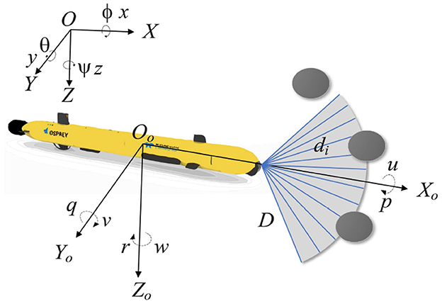

Figure 1. Schematic representation of the variables of the AUV motion model and the sonar model.

In a 2D environment, the effects of the AUV's roll and pitch can be neglected (Song et al., 2016), so ϕ, θ and w are zero, the simplified two-dimensional kinematic model is represented as follows:

{ẋ=ucosψ-vsinψẏ=usinψ+vcosψψ˙=r.    (2)

This simplified model effectively describes the AUV's planar motion, facilitating trajectory planning and control design.

2.2 Sonar model

During underwater missions, AUV frequently encounters complex environments such as reefs, schools of fish, and unknown obstacles. To navigate safely, AUV relies on sensors to detect their surroundings and provide data to the planning algorithm. Ranging sonar (Wang and Yang, 2013), known for its simplicity and low cost, is the most widely used underwater detection device. It emits a conical beam and calculates the distance to obstacles by measuring the time difference between transmitted and received beams. When multiple ranging sonars are combined into a multi-beam sonar, they cover a sector-shaped area in front of the AUV.

We assume that the bow of the AUV is equipped with 12 ranging sonars, each with an aperture angle of 10°, providing a horizontal coverage span from −60° to 60°. Figure 1 shows the detection area, where D is the maximum detection range. di is the distance to an obstacle in the beam direction. If no obstacles are detected by one of the ranging sonars, then di = D. The detected distances are recorded in a 1x12 matrix M = [d1, d2, …, d12].

2.3 Reinforcement learning

Reinforcement learning relies on the framework of Markov Decision Processes (MDPs) to model the interaction between an agent and its environment (Alvarez et al., 2004). MDPs are defined by five key components: the state space S, the action space A, the state transition probabilities P, the reward function R, and the policy π(a|s), which represents the probability of taking action a in state s (Alvarez et al., 2004). In each iteration, the agent selects an action at based on its current policy πt, which influences the state transition of the environment. This leads to a new state st+1 and an associated reward rt from the environment, resulting in an interaction experience (st, at, rt, st+1) (Hossain et al., 2023). By gathering these experiences, the agent gradually enhances and refines its policy. The decision-making process is illustrated in Figure 2.

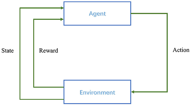
Figure 2. Reinforcement learning control process.

The cumulative discounted reward (Knox and Stone, 2012) represents the total reward that can be obtained over all future time steps after taking action in a given state. In the case of finite time steps, it can be expressed as:

Ut=rt+γrt+1+γ2rt+2+⋯+γT-trT=∑k=0T-tγkrt+k,    (3)

where γ denotes the discount factor used for calculating the present value of future rewards, which takes a value between 0 and 1. Ut accumulates all future rewards from time step t to the terminal time step T.

In reinforcement learning, the action-value function and state-value function are two central concepts. The action-value function Qπ(st, at) evaluates the value of taking an action a in state s and later acting according to strategy π. The state-value function Vπ(st), on the other hand, does not depend on a specific action but rather evaluates the expected payoff that can be obtained when starting from state s and always following strategy π (Li W. et al., 2021). They are formulated as follows:

Qπ(st,at)=?at~π(at∣st)[Ut∣st,at],    (4) Vπ(st)=?at~π(·∣st)[Ut∣st].    (5)

To estimate the value function in a continuous state space, the Deep Q-Network (DQN) incorporates neural networks, which use Qπ(st, at; δ) to approximate the estimate of Qπ(st, at), where δ denoting the parameters of the neural network (Gao Y. et al., 2021). DQN further includes a target network Qπ′(st+1,at+1;δ′), whose parameters are periodically updated from those of the current network, to estimate the maximum value of the subsequent state-action pair. Following is the computation of the DQN loss function:

Loss=?[(r+γmaxat+1Qπ′(st+1,at+1;δ′)-Qπ(s,a;δ))2].    (6)

The introduction of the target network in DQN enhances its efficiency and convergence, reducing variance during training and stabilizing the learning process.

2.4 Dueling Double Deep Q-Network

Merging the advantages of Double DQN with those of Dueling DQN results in the formation of the Dueling Double Deep Q-Network (D3QN) algorithm. This integration addresses the overestimation bias typically found in the conventional DQN, thereby enhancing the learning process's overall performance and stability. Double DQN separates the action selection from the target Q-value computation by identifying the action with the highest Q-value in the current Q network and then using this action to calculate the target Q-value in the target Q network, effectively reducing the risk of overestimation (Hasselt et al., 2016). Here is the definition of the loss function:

Loss=?[(r+γQπ′(st+1,argmaxat+1Qπ(st+1,at+1;δ);δ′)-Qπ(s,a;δ))2],    (7)

where argmaxat+1Qπ(st+1,at+1;δ) denotes the selection of an action at+1 from the current Q network that maximizes the Q value in state st+1.

The Dueling DQN algorithm decomposes the Q-value function into two separate components: one representing the state value and the other encapsulating the advantage. The state value function estimates the expected return for a particular state, while the advantage function quantifies the benefit of taking a specific action compared to the average performance in that state. This separation enhances the accuracy of state value assessments and the evaluation of action benefits, leading to improved model efficiency and performance. The Q-value in Dueling DQN is computed as follows:

Qπ(s,a;δs,δa)=(A(s,a;δa)-1|A|∑ai∈AA(s,ai;δa))+Vπ(s;δs),    (8)

where Vπ(s; δs) denotes the state value function, A(s, a; δa) represents the advantage function, and |A| denotes the total number of possible actions. By integrating the enhancements from these two algorithms, we can formulate the corresponding loss function for D3QN as follows:

Loss=?[(r+γQπ′(st+1,argmaxat+1Qπ(st+1,at+1;δs,δa);δs′,δa′)              −Qπ(s,a;δs,δa))2]    (9)

D3QN has demonstrated superior performance in various applications compared to traditional DQN, establishing it as a leading algorithm in reinforcement learning (Gök, 2024).

3 Methods

This section provides a detailed introduction to the ND3QN algorithm. Initially, we describe the environmental state variables, including AUV position and orientation information, obstacle information, and ocean current data. Subsequently, we expand on the action space and describe the state transition method. Following this, we elaborate on the composite reward function, which accounts for factors such as ocean currents, obstacles, and turning constraints. Lastly, we introduce a noise network based on the D3QN algorithm.

3.1 Environmental states

In the realm of reinforcement learning research and applications, environmental state variables form the foundation of an agent's perception of the surrounding environment. These variables constitute a set of observational data, thereby providing a comprehensive representation of the agent's context, which is crucial for the agent to make effective decisions (Sutton and Barto, 2018). In the underwater operational environment of an AUV, the environmental state variables should encompass the AUV's position and orientation information, as well as external elements like ocean currents and obstacles. In this study, the AUV's local environmental information is represented by the state variables S=[ξ→xy,ψ,∇→cur,M], where ξ→xy denotes position information, ψ represents heading angle information, ∇→cur indicates ocean current information, and M denotes the detection range matrix.

3.1.1 Position orientation information

To enhance the model's ability to generalize, we convert absolute position coordinates into relative position vectors. Assuming the current position coordinates are P(x, y) and the goal position is Pgoal(xgoal, ygoal), the vector representation of the current position and goal coordinates is given as:

ξ→xy=(xgoal-x,ygoal-y).    (10)

The AUV's decision-making will be influenced by its attitude differences, even when it is in the same circumstance. Therefore, we incorporate the AUV's heading angle ψ as attitude information into the environmental state variable.

3.1.2 Information on external environment

In complex ocean environments, the movement of an AUV is influenced by ocean currents. In real data formats, ocean current information is typically provided as gridded data. Therefore, interpolation is needed to estimate the discrete ocean current data. The ocean current value ∇→cur at P(x, y) can be interpolated from the current values at its four neighboring grid points Poj (xoj, yoj), where oj = 1, 2, ..., 4, as follows:

∇→cur=∑∇→curoj·Leuc(P,Poj)∑Leuc(P,Poj),    (11) Leuc(P,Poj)=(x-xoj)2+(y-yoj)2,    (12)

where Leuc(P, Poj) defines the Euclidean distance between two points P(x, y) and Poj (xoj, yoj).

The detection range matrix M = [d1, d1, …, d12] can be obtained through a sonar ranging model, allowing the AUV to perceive detailed information about surrounding obstacles.

3.2 Action space and state transition function

Some of the existing AUVs can only rotate at fixed angle increments instead of arbitrary angles during navigation, as their steering rudders are limited by factors such as mechanical structure, motor characteristics, and control system. Therefore, in this paper, the navigation direction of AUV is designed as a discrete action. To broaden the range of directional options available for an AUV, we have discretized its horizontal movements into 16 distinct actions, a = [a1, a2, a3, ..., a16], each separated by an angle of 22.5, as illustrated in Figure 3. Compared to the existing options of 6 (Xi et al., 2022) or 8 (Yang et al., 2023a) actions, the availability of 16 actions offers a finer