1 Introduction

Intelligent systems acquire information about their surroundings by engaging in contextual scene learning, which entails establishing connections among different environmental components. The system collects, evaluates, and interprets visual data from its environment to provide relevant and context-specific clues for understanding the situation. The framework can assess contextual scene learning and identify objects by detecting the spatial and semantic connections between objects and eliminating their features. This will facilitate the transition of systems from understanding to resilience and context awareness. Song et al. (2015) introduced the SUN RGB-D dataset, which provides a comprehensive benchmark for RGB-D scene understanding, highlighting the necessity of multi-modal data for accurate scene interpretation. This work highlights the challenges in integrating multiple data types to enhance object recognition and scene comprehension.

There has been a recent increase in interest in developing computational frameworks that can comprehend the complexities of vast quantities of visual data. Computerized systems with the ability to accurately identify objects and determine their importance in a certain situation are essential for augmented reality, surveillance, and autonomous vehicles (Rabia et al., 2014; Murugan et al., 2022; Ghasemi et al., 2022). Optimal results require innovative approaches to managing several situations within a specific setting.

The current investigation introduces a novel approach known as Deep Fused Networks (DFN) to tackle these issues. DFN, in contrast to traditional approaches, seeks to integrate several sophisticated methodologies by leveraging the capabilities of deep learning to overcome their limitations. The primary objective is to enhance accuracy in identifying many items in challenging conditions. DFN is a reliable framework for object detection that effectively combines several models by emphasizing their distinctive qualities. This novel methodology facilitates the identification of items in intricate scenarios characterized by factors such as partial concealment (occlusion), alterations in size, and crowded backdrops. Moreover, and perhaps most significantly, DFN facilitates a comprehensive comprehension of visual images by analyzing their underlying meaning. This framework utilizes the context of existing objects to extract more advanced information, such as scene characteristics, object relationships, and item categorization within the scene or environment.

Contextual scene understanding has drawn a lot of interest lately because of its vital uses in robotics, autonomous vehicles, and surveillance. Due to the inherent constraints of a single modality, traditional approaches that rely merely on RGB (color), images frequently struggle to appropriately interpret complex scenarios. For example, it can be difficult to discriminate between objects, like a red ball on a red carpet, that have identical colors but different textures or depths. Our proposed approach uses multi-modal data—that is, RGB and depth (RGB-D) information—to overcome these challenges. We can capture both the geometric and visual aspects of the scene by combining RGB images with depth information, which results in a more accurate and robust contextual understanding. By incorporating multi-modality, we have addressed the following important challenges:

i. Multi-modal data helps in discriminating objects that appear similar in RGB images but have distinct geometric properties.

ii. Depth information aids in identifying partially occluded objects, providing a clearer understanding of the scene.

iii. Combining RGB and depth data enriches the feature set, allowing for better semantic segmentation and scene understanding.

This comprehensive analysis enhances comprehension of the visual context and facilitates more informed decision-making. To evaluate the effectiveness of our proposed DFN framework, we conducted experiments using established benchmark datasets and conducted a comparative analysis with other existing approaches. The results of our studies indicate that the DFN model is both robust and successful since it achieved gains in both multi-object identification accuracy and semantic analysis. To summarize, this research proposes a complete strategy to address the difficulties of achieving dependable multi-object detection and semantic analysis to enhance scene comprehension. The suggested Deep Feature Network (DFN) enhances both the effectiveness of object detection and the comprehension of visual situations, hence creating new opportunities for diverse computer vision applications.

• Deep Fused Network for Scene Contextual Learning through Object Categorization: The study introduces a deep-fused network that facilitates scene contextual learning by incorporating object categorization.

• FuseNet Segmentation: The study presents FuseNet segmentation which is a unique approach that utilizes deep learning techniques to achieve precise and efficient semantic segmentation. FuseNet combines multi-scale features. It also utilizes fully convolutional networks to improve the accuracy of segmentation results.

2 Literature review

Multi-object detection and semantic analysis in complex visual scenes have been active areas of research in the field of computer vision. In recent years, deep learning techniques have revolutionized these domains by achieving remarkable performance improvements. Various deep learning-based object detection methods have been proposed, such as Faster R-CNN (Pazhani and Vasanthanayaki, 2022) YOLO (You Only Look Once) (Diwan et al., 2023) and SSD (Single Shot MultiBox Detector) (Ahmed et al., 2021). These methods leverage convolutional neural networks (Dhillon and Verma, 2020) have challenges dealing with complex scene scenarios, occlusions, and object changes. Researchers are investigating different methods to strengthen object detection’s robustness to overcome these issues (Zhang et al., 2023), presented automated systems with the ability to accurately detect objects and determine their importance in a certain situation are essential for augmented reality, surveillance, and autonomous vehicles (Silberman et al., 2012), in their work on the NYU-Dv2 dataset, demonstrated how combining RGB and depth data can significantly improve object detection in indoor environments, addressing issues like occlusion and varying object scales. This sets the stage for our proposed approach, which aims to integrate and improve upon these methodologies.

One approach involves integrating different detection models to create a more precise system. Fusion can occur at various levels, such as feature-level fusion (Liu et al., 2017; Xue et al., 2020; Wang et al., 2020), decision-level fusion (Seong et al., 2020), or both. These fusion-based solutions aim to enhance detection accuracy and handle challenging scenarios by leveraging the strengths of multiple models. On the other hand, semantic analysis focuses on capturing high-level semantics and understanding the context of objects within an image. This research considers the categorization of objects, relationships between objects, and scene components. Unlike traditional methods relying on hand-crafted features and rule-based procedures, which have limitations in capturing complex contextual data, researchers can now utilize deep neural networks for a more comprehensive and accurate semantic analysis, thanks to advancements in deep learning.

This research proposed a unique framework called Deep Fused Networks (DFN) to support contextual scene learning. DFN provides a consistent and reliable recognition system by fusing the benefits of many object detection methods. DFN integrates several models to handle complicated scenarios like occlusions, scale variations, and crowded backgrounds. DFN also uses semantic analysis to draw out stronger semantics from visual scenes. By utilizing contextual information, the framework enables comprehension of scene attributes, object associations, and object categorization. This in-depth research enables a deeper comprehension of visual scenes and enhances decision-making.

2.1 Multi-object segmentation

Machine learning has been used in computer vision tasks for years, particularly in advanced applications like detecting multiple objects, recognizing scenes, and understanding contextual scenes. Numerous researchers have dedicated their efforts to exploring the visual aspects of these tasks. In Feng et al. (2020) provide a comprehensive discussion of the latest approaches and challenges in multi-modal object recognition and semantic segmentation for autonomous driving. The authors delve into the methodology, including techniques beyond deep learning, and the various datasets available for training and evaluating such systems. The paper emphasizes the complexity and challenges of these tasks within the realm of autonomous driving. In Ashiq et al. (2022) describe how developing a neural network-based object detection and tracking system can help those who are visually impaired. The authors explain how deep learning techniques are used for real-time object tracking and recognition, allowing users to intelligently navigate their surroundings. The research illustrates how this approach can improve the independence and mobility of people who are visually impaired. It offers a perceptive comprehension of how advanced technology might be applied to improve the quality of life for people with visual impairments. In Zeng et al. (2022), a new approach focused on the detection of imperfections and small-sized objects is presented by N. Zeng et al. To address the specific challenges involved in recognizing small objects, the authors suggest a multi-scale feature fusion method. They focused on the limitations of existing approaches for dealing with small objects and present an alternative that makes use of the fusion of multi-scale features to increase detection accuracy. In this paper, the authors tried to highlight the efficiency of their proposed framework by conducting experiments and an evaluation process for detecting defected objects. In Kong et al. (2022), a lightweight network model named YOLO-G is introduced by L. Kong et al. to improve the system of military target detection. They considered the challenges while improving the target detection accuracy. They presented the simplified form of the “You Only Look Once” (YOLO) technique with some modifications in accordance with the military applications. In Guo et al. (2023) the challenge of scale variation in object detection, by introducing the Multi-Level Feature Fusion Pyramid Network (MLFFPN), which effectively fuses features with different receptive fields to enhance object representations’ robustness. It utilizes convolutional kernels of varying sizes during feature extraction, reconstructs feature pyramids through top-down paths and lateral connections, and integrates bottom-up path enhancement for final predictions. In Solovyev et al. (2021) proposed based on, weighted boxes fusion, introduces a novel method for fusing predictions from various object detection models, emphasizing the utilization of confidence scores to construct averaged bounding boxes. In Cheng et al. (2023) the author addresses the challenge of accurate multi-scale object detection in remote sensing images, by getting inspiration from the YOLOX framework and proposes the Multi-Feature Fusion and Attention Network (MFANet). By reparametrizing the backbone, integrating multi-branch convolution, attention mechanisms, and optimizing the loss function, MFANet enhances feature extraction for objects of varying sizes, resulting in improved detection accuracy. In Oh and Kang (2017) accurate object detection and classification is achieved through decision-level fusion of classification outputs from independent unary classifiers, leveraging 3D point clouds and image data. The approach utilizes a convolutional neural network (CNN) with five layers for each sensor, integrating pre-trained convolutional layers to consider local to global features. By applying region of interest (ROI) pooling to object candidate regions, the method flattens color information and achieves semantic grouping for both charge-coupled device and Light Detection And Ranging (LiDAR) sensors. In Xiong et al. (2020) the author introduces a novel fusion strategy, BiSCFPN, based on a backbone network. Comprising bi-directional skip connections (BiSC), selective dilated convolution modules (SDCM), and sub-pixel convolution (SP), this strategy aims for simplicity and efficiency in high-quality object detection. BiSCFPN aims to mitigate the problems associated with traditional interpolation methods and strives to achieve a better balance between precision and speed, addressing limitations observed in current approaches.

2.2 Contextual scene learning

In the past, semantic segmentation for object detection and contextual scene learning has been performed manually. However, the advancement in deep learning-based image-processing techniques has improved computer vision tasks nowadays. These advanced approaches are critical to extracting complex contextual information from images, enabling more precise and efficient object detection for contextual scene-learning tasks. In Kim et al. (2020) explores the use of contextual information to improve the accuracy of monocular depth estimation. While addressing the limitations of depth estimation from a single image, the authors propose a framework that incorporates contextual cues such as object relationships and scene understanding. The framework provides detailed information over contextual information with reference to its potential for advancing monocular depth estimation techniques. In Dvornik et al. (2019) demonstrates the significance of incorporating visual context during data augmentation to enhance scene understanding models. To understand the contextual relationship between the objects they improved the robustness and generalization capabilities of the models. In Wu et al. (2020) emphasize combining pyramid pooling and transformer models to enhance the efficiency of scene understanding tasks under specific conditions. They overcame the limitations of existing methods in capturing both local and global contextual information within scenes. The authors propose P2T as a solution to effectively incorporate multi-scale features and long-range dependencies for comprehensive scene understanding. In Hung et al. (2020) the authors introduce the Contextual Translation Embedding approach, which incorporates contextual translation to improve the accuracy and contextual understanding of visual relationships. They contribute to the field of detecting visual relationships and scene graph generation. Additionally, they offer possible developments in capturing fine-grained details and spatial patterns within visual scenes. In Chowdhury et al. (2023) a unique approach is introduced by extending the representation to encompass human sketches, creating a comprehensive trilogy of scene representation from sketches, photos, and text. Unlike rigid three-way embedding, the focus is on a flexible joint embedding that facilitates optionality across modalities and tasks, allowing for versatile use in downstream tasks such as retrieval and captioning. Leveraging information-bottleneck and conditional invertible neural networks, the proposed method disentangles modality-specific components and synergizes modality-agnostic instances through a modified cross-attention mechanism, showcasing a novel and flexible approach to multi-modal scene representation. In Hassan et al. (2020) novel approach is introduced by integrating handcrafted features with deep features through a learning-based fusion process, aiming to enhance detection accuracy under challenging conditions such as intraclass variations and occlusion. This work builds upon the YOLO object detection architecture, aligning with the contemporary trend of leveraging deep learning methods for improved object localization and recognition in complex real-life scenarios.

The summary of the above studies has been incorporated with all the required fields in a table to clearly elaborate the findings and limitations of the existing studies as follows:

3 Materials and methods 3.1 System methodology

In this section, we present our methodology for contextual scene learning using a multi-stage approach. The process is comprised of multiple steps. Initially, we start with the input acquisition, followed by preprocessing to enhance the quality and consistency of the data. We then employ the FuseNet segmentation network to extract pixel-wise semantic information from the input images. Next, feature extraction and fusion through various techniques from multiple modalities, comprehensive information is acquired to proceed with object categorization. Subsequently, to assign the semantic labels to each individual object within the scene, object categorization is incorporated. Once the objects are classified into various categories, object-to-object relationship modeling is then employed to gather the contextual information of these objects. Finally, a fully convolutional network is employed for contextual scene learning, enabling a holistic understanding of the scene and its semantic context as shown in Figure 1.

Figure 1. Schematic view of the proposed model for contextual scene learning.

3.2 Pre-processing

In the context of RGB and depth images used for scene understanding, noise is commonly observed during pre-processing, particularly in regions with low texture or reflective surfaces. To minimize the effects of noise on further analysis, noise reduction techniques are employed. Among these techniques, Gaussian or bilateral filtering methods (Zhang and Gunturk, 2008) are frequently applied to depth images. These techniques are effective in effectively reducing the presence of noise and smoothing images while preserving essential structural information. Mathematically, we can express the bilateral filter as follows (see Equation 1):

B(x,y)=(1W(x,y))∑i,j∈Ω(x,y)I(i,j)GSpatial(||(x,y)−(i−j)||)GIntensity(|I(x,y)−I(i,j)|)    (1)

where (x,y) denotes the coordinates of the pixel being filtered, (i,j) means the coordinates of the neighboring pixel, Ω(x,y) means neighborhood pixels around pixel (x,y) , I(x,y) is the intensity value of the neighboring pixel, GSpatial is the spatial Gaussian kernel that captures the spatial proximity between pixels, GIntensity is the intensity Gaussian kernel that measures the similarity of pixel intensities, W(x,y) is the normalization factor that ensures the sum of weights is equal to 1 and can be expressed as (Equation 2):

W(x,y)=∑i,j∈Ω(x,y)GSpatial(||(x,y)−(i−j)||)GIntensity(|I(x,y)−I(i,j)|)    (2)

The bilateral filter is effective in different aspects when compared with the Gaussian filter. Specifically, it is superior in terms of preserving edge information while removing noise from the input image. The bilateral filter considers both the spatial proximity and pixel intensity differences during the noise removal or smoothing process.

3.3 FuseNet segmentation

The FuseNet method, designed for semantic segmentation and understanding contextual scenes which combines RGB and depth information to label each pixel in a scene accurately. Its goal is to capture features based on both appearances from RGB images and geometric aspects from depth information, enhancing the accuracy of segmentation. The FuseNet architecture typically involves two branches: the RGB branch and the depth branch. Each branch processes the respective input modality and extracts relevant features. The output feature maps from both branches are then fused together to generate the final segmentation result as shown in Figure 2 using Equations 3, 4.

FRGB=MaxPool(IRGB,Ksize=3, St=2)    (3) FDepth=MaxPool(IDepth,Ksize=3,St=2)    (4)

where FRGB denotes the RGB features while FDepth means the depth features, extracted by RGB and depth branches of FuseNet Segmentation architecture, respectively. FRGB and FDepth represent the downsampling of features obtained from the RGB and depth branches, achieved through the MaxPool operation. The MaxPool operation involves traversing the input features with a 3×3 kernel, selecting the maximum value within each region, and moving with a stride of 2, indicating the number of pixels the kernel shifts during each step. These operations result in down-sampled feature maps that capture essential information while reducing spatial dimensions. The fusion of the feature maps may be expressed mathematically as follows using (Equation 5):

FFused=WRGB∗FRGB+WDepth∗FDepth    (5)

where WRGB is the weight assigned to RGB images, while WDepth represents the weights assigned to depth images. Similarly, * denotes the element-wise multiplication for fusion, and + denotes the element-wise addition. The general FuseNet process can be represented mathematically as follows (see Equation 6):

S=FuseNet(IRGB,IDepth)    (6)

A commonly used initial learning rate is 0.01. However, with the passage of time and an increasing number of epochs that reduce the learning rate to adaptively adjust the learning rate during training based on the model’s performance. FuseNet consists of 6 convolutional layers interleaved with pooling layers. However, the depth of the network can be adjusted based on the complexity of the RGB-D datasets and the available computing resources. Moreover, we use 3×3 filters in the convolutional layers to capture the local context. Strides of 2×2 are used in pooling layers for down-sampling and spatial resolution reduction. For semantic segmentation of RGB-D datasets, the combination of cross-entropy loss and Dice loss is used as described in Equations 7, 8, respectively.

LCE=−∑i=1nyilog(pi)    (7) LDICE=1−2∗∑i=1n(yipi)/(yi+pi)    (8)

where yi denotes the ground truth label while pi represents the predicted probability for pixel i, respectively. The cross-entropy loss helps to optimize the pixel-wise class predictions, while the Dice loss encourages better overlap between the predicted and ground truth segmentation masks. The relative weight between these losses can be adjusted based on the dataset characteristics. The results of FuseNet segmentation are demonstrated in Figure 3.

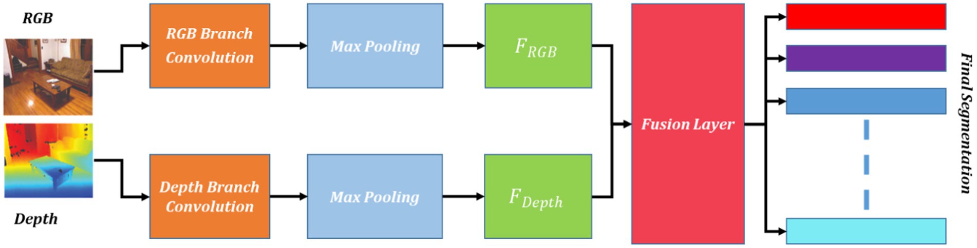
Figure 2. Schematic view of FuseNet segmentation.

Figure 3. Results of FuseNet segmentation over some images from the SUN-RGB-D dataset. (A) Original images and (B) segmented images.

3.4 Feature extraction

To extract the deep features from segmented objects are taken as input and can be expressed as follows segmentation. We can identify regions with similar color or texture characteristics by grouping similar pixels into clusters, which can then be used as inputs for region-based segmentation (see Equation 9).

SObj∈ℝ^(H×W×C)    (9)

where H and W denote the height and width of the segmented image, respectively. While C represents the number of channels. Each pixel of the segmented object can also be represented as SObj(i,j,k) where i,j are the coordinates of the segmented image, and k denotes the index of the channel. The input is processed for convolution over the convolution layer where filters (kernels) are used. These filters are denoted by weight matrix Wm having a size F×F×CPre where F represents the size of the filter, and CPre is the number of channels from the previous layer. The convolution process is computed mathematically as follows (Equation 10):

Fm_con=Af(Wm,SObj+b)    (10)

where Af represents the activation function, Fm denotes the output feature map of the convolutional layer, Wm is the weight matrix, SObj is the input of the layer, which is segmented objects, and b denotes the bias. The output feature map is forwarded to the pooling layer to reduce its dimensions by converting the overlapping regions into non-overlapping regions. The size of regions is defined by P×P . After the dimensions are reduced from the pooling layer, the feature map has the following dimensions (see Equation 11):

(Wpool,Hpool+Cout)    (11)

where Hpool is the height, Wpool is the width of the output feature map of the pooling layer and Cout is to denote the number of channels. The feature maps obtained from convolutional and pooling layers are flattened into a single dimension as a vector to serve as input to the fully connected layer.

The decoder is used to reconstruct the encoded feature maps to the original resolution of the input image. This process involves transposed convolutions (deconvolutions) to up-sample the feature maps. The goal of the decoder is to generate high-resolution feature maps that accurately represent the spatial context and details of the original segmented objects. The details are as follows:

The encoder outputs a feature map of size 16 × 16 × 128 (height, width, channels). Apply a transposed convolution with a filter size of 3 × 3, a stride of 2, and appropriate padding. This operation up-samples the feature map to 32 × 32 × 64. Then another transposed convolution with similar parameters is applied that up-sample the feature map to 64 × 64 × 32. Finally, a transposed convolution to match the original input image resolution is applied that will up-sample the feature map to 128 × 128 × 3. The schematic view of feature extraction using CNN is demonstrated in Figure 4.

Figure 4. Schematic diagram of feature extraction using CNN.

3.5 Object categorization via MLP

For the MLP architecture, we designed a two-layer fully connected network. The first hidden layer consists of 512 neurons, followed by a ReLU activation function to introduce non-linearity. The second hidden layer consists of 256 neurons, also followed by a ReLU activation function. The output layer contains as many neurons as the number of object categories in the SUN RGB-D dataset, with a softmax activation function to generate class probabilities. Figure 5 illustrate the details of object categorization.

Figure 5. Schematic diagram of object categorization using MLP.

The neurons in the layers of MLP can be expressed as by using Equation 12 as follows:

yij=f(∑(Wij∗Xij+bij))    (12)

where yij is the output, Xij is the input of the ith neuron at layer j , while Wij denotes the weights associated with these inputs, bij is to represent bias and f is the activation function applied to the weighted sum. To update the weights Wij (Equation 13), the following backpropagation is used:

ΔWij=−η∗∂E/∂Wij.    (13)

where ΔWij the rate of change in weights is, η is the learning rate, E is the total error and can be written as E=LCE+LDICE , and ∂E/∂Wij denotes the partial derivative of the error with respect to the weight Wij . The object categorization results are presented in Figure 6.

Figure 6. Object categorization results by applying MLP over the SUN RGB-D dataset.

3.6 Object–to–object (OOR) relationship

Graph-based object-to-object relationships (Hassan et al., 2020) provide a powerful setting for contextual scene learning, enabling a structured representation of the relationships and interactions between objects within a scene. To understand a scene comprehensively, objects are modeled as nodes having attributes such as their semantic label, position, and size while their relationships are considered as edges. These relationships can be classified into different types, such as containment, proximity, support, or interaction during scene understanding tasks or contextual scene learning.

To construct the object-to-object relationship graph, a technique to analyze the spatial attributes of categorized objects Obj , considering factors such as distance, overlap, or relative positions is applied. Let us consider OOR graph as general graph G=VE where V means the set of nodes or detected objects Obj while E denotes the set of edges or relationships between these categorized objects, and G is equivalent to OOR which is the relationship between these objects. The relationship between objects can be expressed as an adjacency matrix as described in Equation 14 below.

A∈^(|Obj|×|Obj|)    (14)

where A=1 if there is a relationship between the objects and A=0 otherwise.

Let yI be the scene labels, and OOR be the set of possible semantic relationships between objects. The mathematical function of OOR can be represented as follows (see Equation 15):

OOR=f:Obj→yI    (15)

The contextual scene learning system utilizes the capabilities of graph-based object-to-object relationships to accomplish holistic scene understanding. This mechanism supports higher-level reasoning, object interaction analysis, and contextual inference. Moreover, other vision tasks such as multi-object detection, scene understanding, and contextual scene learning can be expanded and revolutionized.

3.7 Contextual scene learning via FCN

FCN is one of the most used deep learning models from Convolutional Neural Networks that is used to perform multiple tasks including object categorization, semantic segmentation, scene recognition, and classification. There are numerous advantages of the model, however, the fundamental benefit of FCN over other traditional CNNs is its capability to take the input image without resizing constraints and process it accordingly. The FCN architecture is illustrated in Figure 7.

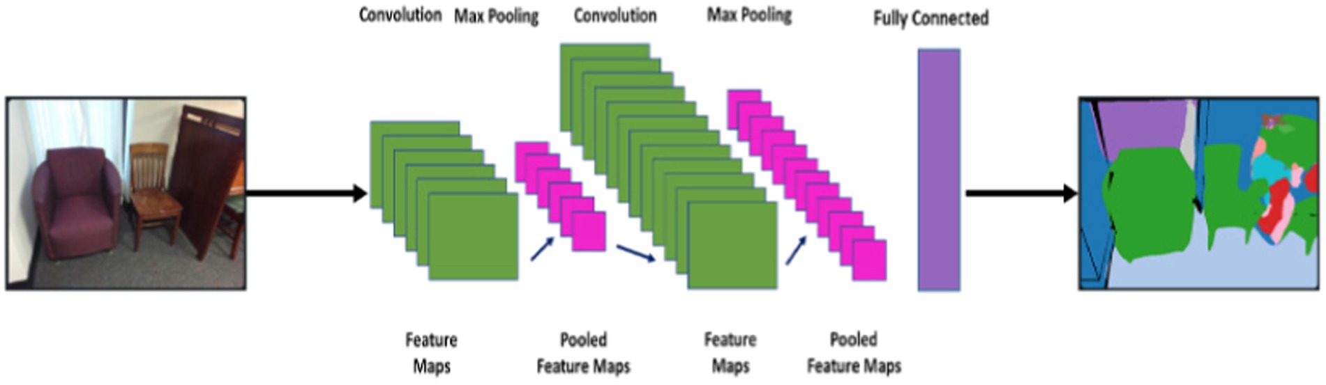
Figure 7. Object categorization results by applying MLP over the SUN RGB-D dataset.

Let us consider in input image (objects) as xI , and the predicted label of the scene as yI . Initially, the FCN is supposed to take xI and the OOR as input and predict scene label yI . The FCN comprised multiple convolutional layers, each of which applies a convolutional filter to the input image. Convolutional filters are learned during training to extract features that are relevant to the task of scene recognition. The OOR relations are a set of pairwise relationships between objects in the scene as computed in the previous section. The OOR relations are used to add additional information to the feature map. Here, is a more mathematical representation of the FCN architecture (see Equation 16):

FCN(xI,OOR)=argmaxyp(yI|xI,OOR)    (16)

where xI denotes the input image features, OOR means object-to-object relations, yI represents the scene label for scene image I, while p(yI|xI,OOR) means the probability of the particular scene label yI when given the input image features xI . The complete flow of the FCN is described in the Algorithm 1.