The hybrid inference in existing literature

BFH inference is designed for models that have both frequentist and Bayesian parameters [45]. Suppose the frequentist and Bayesian parameters are \(\theta_\) and \(\theta_\), respectively, the data is \(}\), and the prior for \(\theta_\) is \(\pi (\theta_ )\). Given a decision \(d\left( } \right)\), a loss function \(W\left( } \right),\theta_ } \right)\), and the distribution likelihood \(f(}|\theta_ ,\theta_ )\), the hybrid estimators of \(\theta_\) and \(\theta_\) are

$$\left( _ ,\check_ } \right) = \arg \inf \sup \int } \right),\theta_ } \right)f(}|\theta_ ,\theta_ )\pi (\theta_ )d\theta_ } ,$$

where \(}\) and \(sup\) were taken in the space of \(d\left( } \right)\) and \(\theta_\) respectively so that \(\check_\) minimizes the posterior risk given \(\hat_\) and \(\hat_\) maximizes the likelihood function given \(\check_\). The frequentist parameter \(\hat_\) is defined (and can be numerically calculated) as integration of the loss function over the posterior distribution. Yuan [45] proved that the hybrid estimator is a consistent estimator, and the standard error of the hybrid estimators can converge to that of the frequentist estimators. As a result, the variance–covariance matrix can be quantified using Fisher information matrix. Han et al. [19] developed an EM computational algorithm to compute \(\left( _ ,\check_ } \right)\) for any loss function ensuring that the hybrid inference is applicable to general practical problems and different data settings. Han et al. [19] demonstrated, in extensive simulation studies, that the hybrid inference based on the EM algorithm can outperform Bayesian inference and frequentist inference. In this paper we adopt the EM algorithm in Han et al. [19] to make inference. Data, statistical models, and more details about the computation are given in section "Introduction of frequentist, Bayesian, and hybrid inference in linear regression with conjugate priors".

Single-cell RNA sequencing methods comparison using semi-synthetic dataset

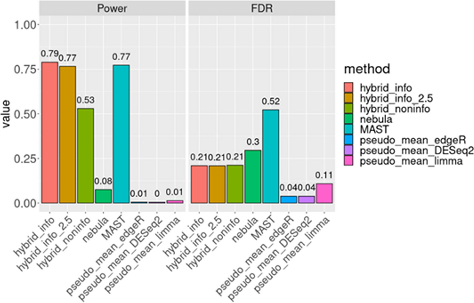
Motivation of semi-synthetic data We employed semi-synthetic data derived from actual single-cell RNA sequencing (scRNA-seq) data to assess the power and false discovery rate (FDR) of our proposed method in comparison to other widely used approaches. Inspired by Li et al.'s work [26], where semi-synthetic data was employed to evaluate bulk RNA-seq differential expression (DE) methods, we sought to extend this approach to scRNA-seq. Traditional simulated datasets often struggle to accurately capture the biological signals and intricate correlation structures present in real datasets, leading to challenges in maintaining cellular population heterogeneity [8]. Consequently, analyses based on diverse simulations and packages may yield conflicting conclusions. For instance, Zimmerman et al. [49] observed superior Type I error rate control and power in mixed models compared to pseudo-bulk methods using simulated data. However, Murphy et al., in a different simulation setup, found that pseudo-bulk methods exhibited the lowest Type II error rate among all tested methods, with equal Type I error rates. Recognizing these discrepancies, we advocate for a more realistic evaluation procedure for DE methods.

Semi-synthetic data source and data generation: HypoMap, a compilation of mouse hypothalamus single-cell RNA sequencing (scRNA-seq) data sourced from 18 publications [35], encompasses 100 normal chow mice, yielding a dataset containing190,710 neuron cells. Given the substantial number of subjects and cells within this dataset, it serves as a valuable resource for generating multiple synthetic datasets. As a subset, 55 mice were identified with a minimum of 1,000 cells each, constituting a total of 170,874 neuron cells. Based on this subset, we derived our semi-synthetic datasets.

In our scRNA-seq semi-synthetic scenario, we randomly selected 20 out of 55 mice. Among these, 10 were arbitrarily assigned to the 'disease' group, while the remaining mice served as the 'normal chow' group. It's important to note that in the original data, the 'disease' group was under normal chow conditions. To achieve around 1,000 cells per mouse, we sampled a specific number of cells from each mouse using a Poisson distribution with a mean of 1,000, ensuring an average of 1,000 cells across the 20 mice.

For the generation of true positives (true differentially expressed genes or true DE genes), we initially focused on genes expressed in at least 10% of the cells, amounting to approximately 8,000 genes. Subsequently, we randomly selected 5% of these genes from the 'disease' group and an artificial fixed effect was introduced to these genes by multiplying the counts under the 'disease' condition by a constant of 2. Consequently, these genes represent true positives, while the remaining genes serve as true negatives (non-DE genes). This process was iterated 100 times to generate 100 semi-synthetic datasets.

Differential expression method selection We carefully selected representative approaches from three domains of previously proposed Differential Expression (DE) methods: mixed models, pseudo-bulk methods, and single-cell methods. Our choice for the mixed model approach was NEBULA [20, 27], edgeR [33], and limma-voom [25].

ScRNA-seq and bulk RNA-seq Data source

Lungmap dataset The Lungmap dataset used in this study was from a published human lung tissue study [39]. The cells were clustered by Seurat v3 [7] and annotated to 31 cell types based on canonical lineage-defining markers. Lungmap dataset served as the reference dataset for Hierarchical XGBoost [9] algorithm to obtain the probability for a cell being an alveolar macrophage cell. In addition to output of probabilities indicating the likelihood of a candidate cell belonging to each individual cell type, HierXGB offers an additional capability. HierXGB can provide cell identity directly using a naive Bayesian approach, assigning the cell type based on the maximum of such predicted probability.

IPF scRNA-seq dataset The idiopathic pulmonary fibrosis (IPF) scRNA-seq dataset was obtained from a previous study on pulmonary fibrosis (PF) disease mechanisms and the corresponding cell types in human lung tissues [17]. This dataset contains over 114,000 cells from 22 donors who had cell observations. Among these 22 donors, 10 are from the control group and 12 from the IPF group. The IPF dataset served as the query data for HierXGB to obtain the probability for a cell being an alveolar macrophage cell.

IPF bulk RNA-seq dataset We also obtained bulk RNA-seq IPF data from human lung tissues [13] in the previous research on the relationship between chronic hypersensitivity pneumonitis and idiopathic pulmonary fibrosis. This bulk IPF dataset contains 18,838 genes from 103 idiopathic IPF samples and 103 unaffected controls samples. For each gene, the mean differences of expression level between the IPF and control groups were calculated using linear regression with the adjustment of age, sex, race, and smoking history. This difference served as the informative prior of the phenotype coefficient.

Data preprocessing of IPF datasets

For scRNA-seq dataset, we selected genes with average expression level across cells greater than 0.1. We removed cells when the number of detected genes was below the lower 2-percentile or with more than 10% of mitochondrial gene expression. For the cell weight calculation, we aligned Lungmap dataset and IPF single cell RNA-seq datasets by their common genes, resulting in 13,988 common genes and 44,294 and 50,383 cells for Lungmap and IPF, respectively. For coefficient estimation of each gene, we matched the IPF scRNA-seq and IPF bulk datasets and obtained 7,886 common genes.

Introduction of frequentist, Bayesian, and hybrid inference in linear regression with conjugate priors

Here, we would like to introduce each of the methods we attempted to identify genes associated with IPF. In linear regression analysis, given the sample size \(n\) and the number of regression parameters \(p\), the data can be arranged in \(Y\) of dimension \(n \times 1\) as the response, and \(X\) of dimension \(n \times p\) as the design matrix. The regression parameter in the model \(\beta\) can be arranged in a vector of dimension \(p \times 1.\)

In our analysis the outcome \(Y\) is the weighted average of a gene’s expression for a particular cell type (e.g., TGF-β1 in alveolar macrophage) at the individual level, \(p\) = 1, and \(X\) the design matrix is composed of a vector of 1 s, \(X_\) the disease group of the individual (control or IPF), and \(X_\) the predictive probability of each cell belonging to alveolar macrophage averaged per individual with subsequent negative log transformation. The linear model is \(Y = X\beta + \varepsilon ,\varepsilon \sim N\left( \sigma^ I} \right)\), where \(I\) is an identity matrix with dimension n by n. So \(Y\sim N\left( \sigma^ I} \right)\). The regression parameters are \(\beta = (\beta_ ,\beta_ ,\beta_ ),\) which \(\beta_ , \beta_\) and \(\beta_\) are the intercept, regression parameter for disease group, and regression parameter for probability of the cell belonging to alveolar macrophage, respectively. The likelihood value given data (\(},}\)) is

$$\small P\left( },}} \right)\beta } \right) = \mathop \prod \limits_^ P\left( = N\left( \beta ,\sigma^ } \right)} \right).$$

(1)

The conjugate prior of the regression parameter can be written as \(\pi \left( \beta \right)\sim N\left( _ ,\Sigma_ } \right).\) Then the posterior distribution can be derived as

$$\small P\left( \left( },}} \right)} \right) \propto P\left( },}} \right)\beta } \right)\pi \left( \beta \right)\sim \mathop \prod \limits_^ N\left( \beta ,\sigma^ Iy_ } \right) \times N\left( _ ,\Sigma_ } \right)\sim N\left( _^ ,\Sigma_^ } \right),$$

(2)

where \(_^ = \left( ^ + X^}} X} \right)^ \left( ^ _ + X^}} Y} \right)\) and \(\Sigma_^ = \left( ^ + X^}} X} \right)^ \sigma^ .\) Without the prior \(\pi \left( \beta \right)\), the frequentist’s estimate and its variance of \(\beta\) can be written as \(_^ = \left( }} X} \right)^ \left( }} Y} \right)\) and \(\Sigma_^ = \left( }} X} \right)^ \sigma^\), which is the ordinary least square estimate.

Finally, following the EM algorithm in Han et al. [19], the hybrid Bayesian analysis can be written in the following iterative procedures:

[Step 1.] Initialize parameters \((\beta_ ,\beta_ ,\beta_ )\) from the frequentist estimates as \(\left( ^ ,\beta_^ ,\beta_^ } \right)\), where \(\beta_\) is the intercept, and \(\left( ,\beta_ } \right)\) are the slope parameters for disease group \(X_\) and the predictive probability of each cell belonging to alveolar macrophage averaged per individual with subsequent negative log transformation \(X_\), respectively.

[Step 2.] Given the current value of frequentist parameters \(\left( ^ ,\beta_^ } \right)\), generate data \(y_^ = y_ - X_ \beta_^ - X_ \beta_^\). From the regression model \(Y^ = X_ \beta_\), obtain \(\beta_^ \right)}}\) as the posterior mean of \(\beta_\), given a conjugate (normal) prior of \(\beta_\).

[Step 3.] Given \(\beta_^ \right)}} ,\) the posterior mean of \(\beta_\), generate data \(y_^ = y_ - X_ \beta_^ \right)}}\). From the regression model \(Y^ = X_ \beta_ + X_ \beta_\), obtain \(\left( ^ \right)}} ,\beta_^ \right)}} } \right)\) as frequentist estimate of \(\left( ,\beta_ } \right)\).

[Step 4.] Iterate steps 2–3 as in EM algorithm.

For frequentist, Bayesian, and hybrid inferences can all generate parameter estimates and the corresponding estimation variances. An estimate and its variance are used to construct a 95% confidence interval (estimate minus and plus 1.96 times of the standard error) and to calculate a p-value from the two-sided test (by calculating a z-score of estimate divided by the standard error) of whether this value is equal 0 or not based on the underlying normal distribution.

Acquiring weights for alveolar macrophage cells using HierXGB method

Alveolar macrophage cells have been recognized to play a crucial role in the pathogenesis of IPF [2, 46]. Rather than analyzing gene expression levels across all cell types, we are specifically interested in the association between gene expression levels and disease group (IPF vs. control) in alveolar macrophage cells. A simple approach to obtain alveolar macrophage gene expression is to take the unweighted average across the annotated alveolar macrophage cells in the original study. However, single-cell data are high-dimensional, and annotations for different cells have varying degrees of uncertainty. To better characterize the alveolar macrophage gene expression levels, we took this uncertainty into account by assigning higher weights to cells that we are more certain of them being alveolar macrophages. We quantified such uncertainty with probabilities of cells being alveolar macrophages calculated by HierXGB method [9].

HierXGB is a supervised machine learning algorithm that aims to classify each single cell in the query dataset into one of cell types from a reference dataset. With a pre-defined cell-type hierarchical tree structure, the algorithm annotates the cell from ancestor to one of descendant subtypes iteratively until reaching the bottom layer. For dataset with a clear cell type hierarchy, including Lungmap, it outperforms other state-of-arts methods in terms of both accuracy and efficiency [9]. We performed a comparative analysis using the same IPF dataset in with singleR [1], a widely used method for scRNA-seq data annotation to demonstrate the usefulness of HierXGB method in our setting.

In the analysis, we first had Lungmap and IPF scRNA-seq datasets aligned using batch effect correction [40]. Then the HierXGB model was trained by Lungmap and produced the predictive probability of a cell belonging to alveolar macrophage for the IPF scRNA-seq data. The obtained probabilities were used as the weights when we combined gene expression across cells to obtain cell-type-specific expression summary for each gene per individual.

Generating predictor \(}_\) based on alveolar macrophage probabilities and outcome Y as the weighted expression average of alveolar macrophage per patient

In our example, we averaged the probability of being in alveolar macrophages across cells within each of the 22 donors and generated a length-22 vector as the predictor \(}_\). A higher \(}_\) indicates that the cells from this donor are more likely from alveolar macrophages. We also used this alveolar macrophage probability to generate outcome Y. For each gene, Y was also a length-22 vector, where the value was the weighted average of counts in this gene across cells. The weights were alveolar macrophage probabilities, and such weighted averages are called pseudo-bulk counts in single cell data analysis. Weighted averages are more robust to different cell numbers per donor. A higher value of Y indicates that this gene expresses highly in alveolar macrophage cells.

Acquiring priors of the contrast between IPF and healthy and other covariates \(\left( } \right)_}\) and their variance–covariance matrix \(}\) ,

We use non-informative priors such as \(\left( \right)\) and \(diag\left( \right)\) for \(_\) and \(\Sigma_^\), respectively, when we have little information on parameters. However, for RNA-sequencing data, bulk RNA-seq data which are characterized by its affordability and wide availability, can serve as good informative priors. Although bulk data may not have the same high-resolution as single-cell data, they still provide the overall expression level of each gene within the targeted tissue. In our analysis, the key parameter is \(\beta_\) for the disease group, and we incorporated bulk RNA-seq into its estimation. For each gene, we used the difference in mean expression levels between IPF and control samples as the prior of \(\beta_\). We obtained the difference from the coefficient of IPF indicator in a linear regression model adjusting for other covariates including age, smoke, sex, and race. We observed that the sample variance of the difference was relatively small compared with the magnitude of the difference. Directly using it as the prior for the variance of \(\beta_\) would result in a very strong prior distribution concentrated around the mean. To offer a prior with more moderate dispersion, we used the squared root of sample variance of difference as the variance for the prior\(.\) For intercept and average negative log expression, we had no prior information and hence kept the non-informative priors for \(\left( ,\beta_ } \right)\).

Pathway analysis based on differentially expressed genes from frequentist, Bayesian and hybrid methods

Pathway analysis is usually performed using a set of selected features, in this case, differentially expressed genes [23]. The goal of the analysis is to identify common biological pathways or networks and analyze how they interact to form biological processes. The analysis typically involves comparing a list of genes of interest to a reference database that contains information about functional categories such as biological pathways, molecular interactions, canonical signaling, disease biomarker and other areas of biomedical knowledge. The analysis determines whether the genes in the list are significantly enriched or depleted in any of the categories, compared with what would be observed by chance. A pathway with significantly enriched genes would yield a significantly small p-value. We further studied pathways based on a gene subset that satisfies the following criteria. For a set of differentially expressed genes detected by each method, cut-off points were set to obtain a gene subset with FDR less than 0.01 and absolute estimated difference greater than 0.585. The reference database we used was the R package metabaser that collects all system biology products including MetaCore, MetaDrug, and others [6, 30]. The final pathways were identified based on a p-value less than 0.05. Please see the top10 and detailed summary of pathways in Table 1 and 2 and supplement material S5 and S6.

Table 1 Top 10 pathways detected by Bayesian, informative method, ranked by qvalueTable 2 Top 10 pathways detected by Hybrid, informative method, ranked by qvalue