The manipulation of animals was approved by the Institutional Animal Care and Use Committee (IACUC) of The Jikei University School of Medicine (Approval No. 2015–019, 2017–049, and 2022–014) and conformed to the Guidelines for Proper Conduct of Animal Experiments of the Science Council of Japan (2006) and the guidelines of the International Association for the Study of Pain [39].

Animals

Male adult C57BL/6 J mice (age; 7–8 weeks old) were obtained from Charles River Laboratories Japan, Inc. (Yokohama, Japan) and were housed on a 12-h light/dark cycle with free access to food and water.

Induction and evaluation of scratching behavior

All mice used in this study underwent 1) implantation of a small magnet ring in the bilateral hindlimb, 2) bilateral hindpaw nail-clipping (the control was nail-intact), and 3) intradermal injection of histamine (the control was saline). The details of these operations are described below.

Implantation of a small magnet

Seven days before the day of scratching recordings (Day 1 in Fig. S1), all mice were anesthetized with isoflurane to shave their nape, insert subcutaneous magnets into the bilateral hind paws, and clip the nails on the bilateral hind paws. Briefly, mice had the skin on the dorsum of the hind paws cut with scissors, a small magnet (1 mm in diameter, 3 mm in length) was inserted with tweezers, and the wound was closed with a bond. This operation did not affect the general behavior of mice.

Nail clipping

Mice were randomly divided into two groups: those with and without clipped nails on the bilateral hindlimbs ("nail-clipped" and "nail-intact", respectively) (Fig. S1, Day1). The nails of all digits on bilateral hind paws were clipped using scissors for mice assigned to the "nail-clipped" group. Nails remained intact in the "nail-intact" group. Mice recovered from anesthesia and were placed into the home cage.

Handling and Habituation

Two days later, mice were handled for habituation to the experimenter for five days (Fig. S1, Day3). Mice were then habituated to the barrel-shaped recording chamber (10.8 cm in diameter, 18 cm in height) used to count the number of scratches for three days. An injection needle was touched against the shaved skin area several times for three days for habituation (Fig. S1, Day5).

Histamine injection and scratching behavior recording

After repeated handling and habituation to the experimenter and recording chamber for one week, mice were further divided randomly into two groups: those for testing the effects of an intradermal injection of histamine and those of saline ("histamine" and "saline", respectively) (Fig. S1, Day 8).

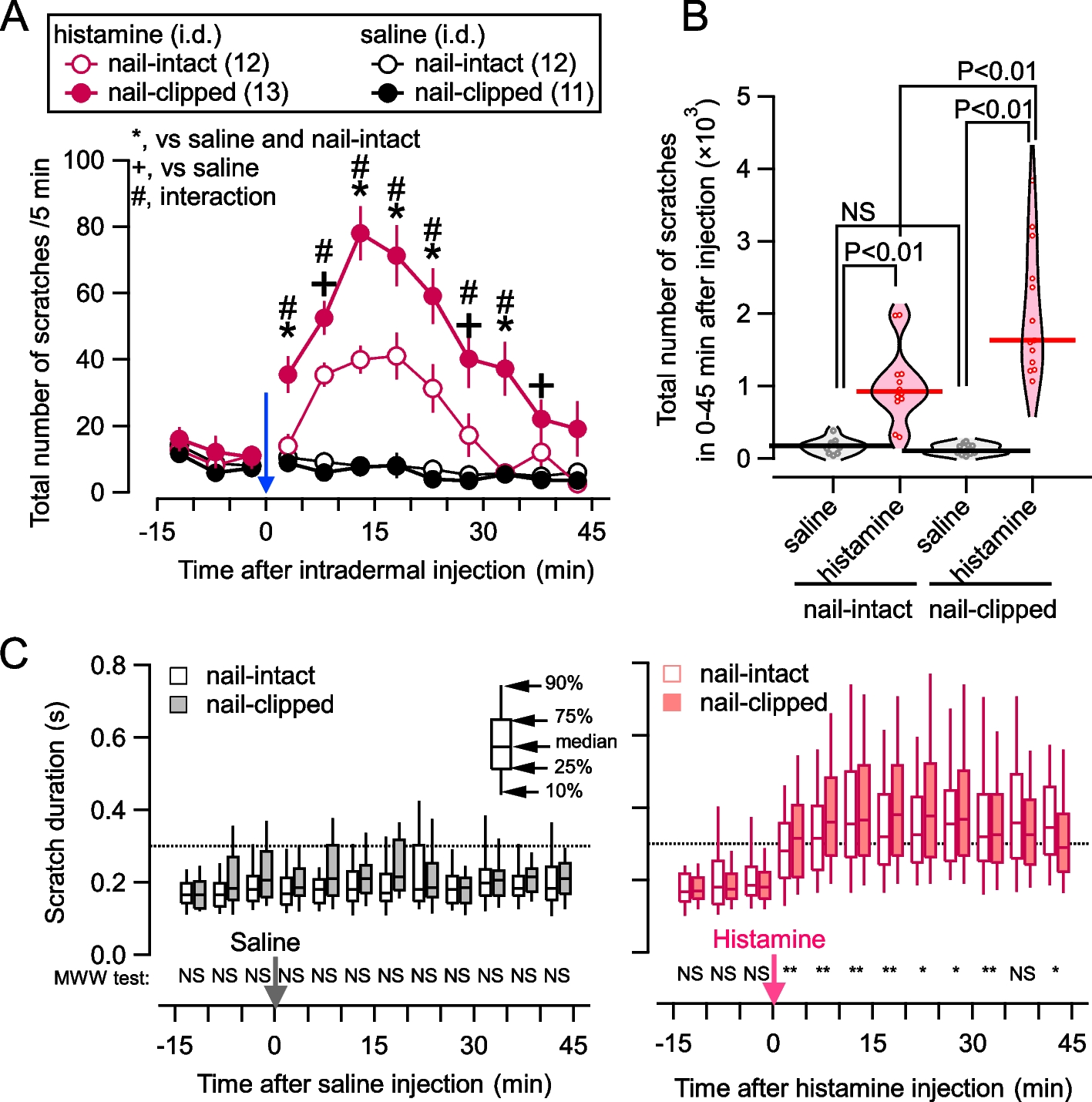
On the day of scratching recording, mice were habituated to the recording chamber for at least 15 min. Mice were removed from the recording chamber and intradermally injected at the nape with histamine (200 μg/20 μL saline; #H7250, Sigma-Aldrich, Tokyo, Japan) or saline (20 μL). Mice were returned to the recording chamber immediately and scratching behavior was recorded for 45 min (Fig. 1A). Scratching behavior was detected using MicroAct® (Neuroscience, Tokyo, Japan). This system is based on the detection of an electric current in the coils according to the movement of the magnets implanted in the hind paws and the measurement of the occurrence time and duration of each scratch bout. After sampling the brain, it was confirmed that magnets remained in both hind paws in all mice (Fig. S1).

The mice cohort size

As described above, all mice used in this study underwent 1) histamine or saline injection and 2) nail-clipping or nail-intact, resulting in four cohorts of mice (Fig. S1). The numbers of mice in each cohort were n = 12 for the histamine-injected + nail-intact group, n =12 for saline-injected + nail-intact group, n =13 for histamine-injected + nail-clipped group, and n =11 for saline-injected + nail-clipped group.

Tissue preparation

Mice were decapitated under 5% isoflurane, and the brain block containing the NAc was dissected and frozen within 5 min. A coronal brain block was freshly frozen using isopentane chilled with dry ice, and stored at -80 °C for up to 2 days. Brain blocks were embedded in OCT compound, and a series of 16-µm-thick coronal sections containing the NAc were prepared with a cryostat (CM1850, Leica Biosystems, Tokyo, Japan). The sections collected were equivalent to the rostrocaudal level from bregma 1.70 mm to 0.86 mm in the Mouse Brain Atlas [40]. Brain sections were stored at − 80 °C for up to 2 days.

Multiplex FISH

FISH was performed using Multiplex fluorescent RNAscope (Advanced Cell Diagnosis [ACD], Hayward, CA, USA; Medical & Biological Laboratories, Tokyo, Japan). The following probes were obtained: Drd1 (Mm-Drd1a-C2, #406,491-C2), Drd2 (Mm-Drd2-C3, #406,501-C3), and Fos (Mm-Fos, #316,921). The RNAscope protocol was followed as indicated in the user manual with adjustments. Briefly, after fixation in 10% neutral-buffered formalin at 4 °C for 15 min, sections were washed with PBS. Sections were then dehydrated in four 5-min dehydration steps in 50, 70, 100, and 100% ethanol. Sections were incubated with protease III (diluted 1:1 with PBS) for 30 min. Fos, Drd1, and Drd2 probes were mixed 50:1:1 and pipetted onto each slide. Probe hybridization and amplification steps were performed according to the standard instructions of the manufacturer. Sections were incubated with DAPI for approximately 30 s, mounted with Aqua Poly/Mount (Polysciences, Warrington, PA) on coverslips, and then stored at 4 °C.

Image acquisition and multiple image alignment (MIA)

All fluorescence images were obtained using the laser-scanning confocal microscope, FV1200 Confocal microscope equipped with 405, 473, 559, and 635 nm laser lines and high-sensitivity GaAsP detectors, with the filter cube FV12-MHYR, using an UPlanSApo 20 × /0.75 NA objective (Olympus, Japan). Multiple overlapping adjacent images of the NAc were taken on a moving stage manually and saved as OIB files (1024 × 1024 pixels). Images of the right side of the brain were captured in this study. A series of OIB files from one brain section were aligned using the MIA function of CellSens imaging software (Olympus, Japan). Multiple images were "stitched" with individual neighboring images into a large "stitched" image without resolution loss by the maximum correlation-based optimization of the software. MIA was performed based on the DAPI channel image (Overlap mode; linear). Each four-channel stitched image was saved as a 16-bit tiff file for subsequent image analysis (Fig. S2A). We positioned images such that the eNAc was dorsal side up and the most medial side was to the right of each image.

ROI definition with the ROI manager in ImageJ

Image data analyses were performed in two steps. The saved tiff file was read by ImageJ/Fiji software (NIH image) for the primary detection of ROIs using the ROI manager. Each of the four channels corresponding to the signals for DAPI, Drd1, Drd2, and Fos in the 16-bit tiff format was read into ImageJ. To detect and register cells, we used DAPI signals by thresholding the DAPI channel image with the Huang method and binarizing using "watershed" separation to prevent detected cells from sticking together (steps 3 and 4 in Fig. S2B). Areas with DAPI signals, likely to correspond to each cell, were numbered and defined as ROIs. The "Analyze Particles" plug-in was applied to these ROIs to measure their characteristics (location, size, and shape properties). We then binarized the signals for the Drd1, Drd2, and Fos channels using Reny entropy methods (step 8 in Fig. S2B) and evaluated the area overlap with each ROI identified according to the DAPI signal using the ROI manager (step 10 in Fig. S2B). At this point, we did not select the detected areas according to the size and circularity of ROIs, which was performed after plotting these features (Fig. S3D). The measured values for Drd1, Drd2, and Fos in individual ROIs were saved in a comma-separated value format together with an 8-bit composite tiff image for further analyses, as described below (step 11 in Fig. S2B).

Expression analysis based on defined ROIs and visualization using a homemade code—"RNAscopeProcessor" on Igor 9

Using the values for each ROI obtained by ROI manager and the original Tiff image, fluorescence signals with each coordinate in slices were identified and analyzed using a homemade code for Igor 9.0 (Wavemetrics).

A composite 8-bit- tiff image of RNAscope that was stitched to cover the accumbens and surrounding structures was loaded together with the results of the ROI manager for each of the three channels (Drd1, Drd2, and Fos). Only apparent artifacts (debris on the slice and tissue overlap) in the image were carefully removed by the drawing tool (Fig. S3A). The detection quality of ROIs was visually confirmed using a zoom-up window showing the tiff image at a higher magnitude with circles showing the diameters of ROIs detected by the particle analysis of ImageJ (white circles drawn on the three-channel image in Fig. S3A and C) and thresholds for the diameter and circularity were fixed with cursors (Fig. S3C and D).

Definitions of zones 1–4, sectors 1–8, and rostro-caudal planes

We defined the following three dimensions to describe the regions of the NAc and surrounding regions (hereinafter called "eNAc"): "zones", "sectors", and "planes".

Defining zones. Concentric circles defining the boundaries between zones were drawn as follows: 1) Circle 1 was drawn around the aco for the boundary between the aco and zone 1. This border was clearly defined because there were almost no neurons within this border, which made it likely to be an outer edge of the region mostly containing rostrocaudally passing axons. 2) Circle 4 was then drawn so that the dorso-medial part of the circle overlapped with the boundary set at the outermost expression of Drd1 and Drd2, forming a border between the NAc and lateral septum nucleus. 3) Two circles (2 and 3) were then positioned between circles 1 and 4 using the observed differences in cell density, which were noted as faint gaps between regions. The radii of these circles are summarized in Table 2. The regions bound by each circle were named Zone 0 (zone within the aco), and Zone 1 (the zone between circle 1 and circle 2), Zone 2, Zone 3, Zone 4, and Zone 5 were then defined accordingly.

Table 2 Summary of radii of five circles used for zone definition Defining sectors

After defining the zones in each plane, eight "sectors" each with a 45° angle, starting from the sector immediately above the horizontal line and most medial (sector 1) and numbered counter-clockwise to sector 8 (Fig. 3), were made.

Defining planes

Three anterior–posterior sections from the rostral, intermed (abbreviated as "intermed"), and caudal NAc were defined (Fig. S3) based on the atlases by Franklin and Paxinos [40] and the Allen Institute [41]. The rostral plane represented (relative to the bregma) 1.78, 1.70, and 1.54 mm coronal sections, the intermed plane, 1.42, 1.34, and 1.18 mm sections, and the caudal plane, 1.10, 0.98, and 0.86 mm sections (Fig. S3E).

With these three dimensions, we classified the eNAc into 96 regions (4 zones × 8 sectors × 3 planes) and performed unbiased analyses of mRNA expression (Fig. S3F). In the Results section, regions were presented with three zone-and-sector plots each for one plane.

Using the results of RNAscope imaging, cells expressing Drd1, Fos, and Drd2 were identified, and thresholds for each signal were selected based on the percentage overlap with the DAPI area. Specifically, Drd1 was defined as positive when overlapping with DAPI by 15% or more, Fos by 20% or more, and Drd2 by 30% or more (Fig. S4A, B, C). The number of cells identified as "positive" for Fos, Drd1, or Drd2 was presented as the fraction of the total number of cells identified with a DAPI signal in each of the 96 regions defined above.

Statistical analysis

Statistical analyses were performed using EZR [42] and Igor 9.0. The total number of scratches were compared using a two-way ANOVA in each timepoint (Fig. 1A) and one-way ANOVA followed by a post hoc analysis with Bonferroni corrections (Figs. 1B). The distribution of the scratch duration in each timepoint was compared using the Mann–Whitney-Wilcoxon test (Fig. 1C). A probability (P) smaller than 0.05 was considered to be significant (Fig. 1A, B, and C). In multiple comparisons of eNAc subregions, P values were corrected using the false discovery rate correction (Benjamini & Hochberg), and corrected values are shown as Q values (Figs. 4A3, 4B3, 5A2, and 5B2). In these cases, t values were presented only for regions with a significance level of Q < 0.1 after false discovery rate corrections (Benjamini & Hochberg). To compare the expression of dopamine receptors, the Kruskal–Wallis test, followed by a post hoc analysis using the Bonferroni correction or the Mann–Whitney U test, was performed (Figs. 4A4, B4, 5A3, and B3). Comparisons of the percentage of dopamine receptors co-expressed with Fos( +) cells were conducted using the chi-squared test (Figs. 4A5, B5, 5A4, and B4). A hierarchical cluster analysis was performed using the values of Fos( +) fractions (Fig. 6) and the Scratch-Fos correlation (Fig. 8) using the hierarchical cluster analysis implemented in Igor 9. We used the Euclidean dissimilarity metric with a Minkowski P value of two. The dendrogram was made with the complete linking method. Spearman's rank correlation coefficients were used in the Scratch-Fos correlation, and P-values < 0.1 were considered to be significant (Fig. 7). Graphs were generated using Igor 9.0 with codes written by one of the authors (F.K.). Analyses were performed by S.I.S. and F.K. in a blinded manner without knowledge of the mouse groups.