This retrospective study with nonequivalent control group study aimed to evaluate the impact of denosumab treatment on various bone parameters derived from DXA in patients with osteoporosis.

We reviewed all KTRs who, upon physician’s decision (based on the clinician’s estimation of fracture risk), started treatment with denosumab 60 mg every six months from January 2014 to January 2018. Patients who received continuous treatment for at least four years, with available baseline and four-year follow-up DXA scans were included.

An untreated cohort was selected among the overall pool of KTRs referring to the clinic who had available baseline and four-year follow-up DXA scans. All KTRs of the denosumab group were then individually age and sex-matched with untreated KTRs with a 1:1 ratio (± 3-year tolerance for age). In the case of two or more potential eligible matches, the closest one in terms of age was selected.

The study therefore included two groups: KTRs treated with denosumab and a control group of age- and sex-matched KTRs not receiving denosumab. Participants were assessed at baseline and during follow-up using DXA to analyze aBMD at the lumbar spine (LS), total hip (TH), and femoral neck (FN). The full details of the protocol, inclusion/exclusion criteria, and the main results including the aBMD data have been published previously [26].

In brief, the study was conducted at the Joint Rheumatology and Nephrology bone clinic, University of Verona (Verona, Italy).

Ten DXA-derived bone were assessed.

TBS T-scores were obtained at the LS at baseline and follow-up for both groups (GE TBS Insight 3.0.3.0). TBS is a texture index that evaluates pixel gray-level variations in the lumbar spine DXA images, providing an indirect measure of bone microarchitecture [27].

3D-DXA analysis at the proximal femur were performed at baseline and follow-up for both groups by 3D-Shaper software v2.11 (3D-Shaper Medical, Barcelona, Spain) as previously described with operators blinded to treatment [21]. Cortical volumetric BMD at Total Hip (Ct.vBMD TH), Trabecular vBMD at Total Hip (Tb.vBMD TH), Cortical vBMD at Femoral Neck (Ct.vBMD FN), Trabecular vBMD at Femoral Neck (Tb.vBMD FN), Cortical surface BMD at Total Hip (c.sBMD TH), Cortical surface BMD at Femoral Neck (c.sBMD FN), Cortical thickness at the Total Hip (Ct.th TH), Cortical thickness at the Femoral Neck (Ct.th FN), and Cross-Sectional Moment of Inertia (CSMI) – Intertrochanteric. were therefore estimated [20, 21].

Student’s t test for independent samples was used to test differences between the two groups and for normally distributed variables, Mann–Whitney U test for non-normally distributed variables, and the chi-square test was used to compare proportions. Paired-samples t tests for each group were conducted to analyze changes versus baseline. To estimate the effect size (ES) of each parameter change for each group, Cohen’s d were also calculated, and interpreted as 0.2 = small effect 0.5 = moderate effect, and 0.8 = large effect [28].

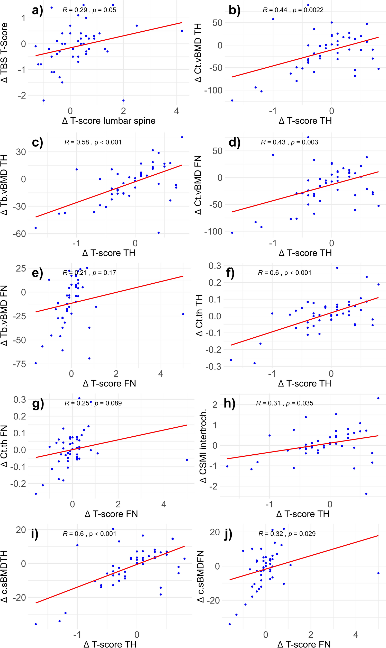
Correlation between each bone parameter and the respective site-specific BMD was tested through Pearson’s correlation. The strength of correlation, expressed as r values, were interpreted as usual: 0.00–0.10 negligible correlation, 0.10–0.39 weak correlation, 0.40–0.69 moderate correlation, 0.70–0.89 strong correlation, and 0.90–1.00 very strong correlation [29].

To assess the effect of denosumab treatment over time and to compare the between-group changes over time of the selected bone parameters, hierarchical linear models were employed. HLMs were chosen due to their ability to handle longitudinal data with repeated measurements, accounting for both inter-individual and intra-individual variability.

For each bone parameter, two distinct nested HLMs were constructed.

1) The reduced model: for each parameter, a model was developed to test the interaction between time (baseline vs. follow-up) and treatment group (denosumab-treated vs. untreated). This model was used to evaluate whether denosumab treatment influenced changes in the bone parameter over time compared to the control group. The general structure of this model was as follows: Parameter∼Time × Group + (1∣Subject ID).

2) The full model: each primary model was further adjusted for the corresponding BMD value at the site of measurement (e.g., total hip aBMD for cortical total hip vBMD). This adjustment was introduced to isolate the unique effect of denosumab on the parameter of interest, independent of BMD changes at the site of observation. The adjusted model accounted for the specific BMD value to control for its potential confounding effect: Parameter∼Site-Specific BMD + Time × Group + (1∣Subject ID).

In both models, patients were clustered by subject (‘Subject ID’) to account for the repeated measures design and to control for intra-individual variability over time. This approach allowed for a more nuanced understanding of the direct impact of denosumab on bone parameters, distinguishing it from changes attributable to corresponding BMD variations, ensuring a more robust evaluation of denosumab’s efficacy on the studied bone parameters, considering both the time-dependent interaction and the influence of site-specific BMD.

Finally, to investigate the potential predictors of aBMD changes over time (expressed as percentage changes from baseline at the lumbar spine, total hip and femoral neck), a Random Forest (RF) model was constructed using the ‘cforest’ function from the party package in R to handle all the predictor variables (measured at baseline) in an unbiased and robust to overfitting manner [30]. The dataset included the following twenty-six variables as predictors: treatment, gender, BMI, presence of type 2 Diabetes Mellitus, concurrent treatment with calcitriol, concurrent treatment with calcitriol cinacalcet, history of fractures, history of pre-transplant dialysis (yes/no), creatinine, ALP, PTH, 25-hydrody vitamin D, serum calcium concentrations (corrected), TBS T-Score LS, Ct.vBMD TH, Tb.vBMD TH, Ct.vBMD FN, Tb.vBMD FN, CSMI intertroch., aBMD LS, aBMD TH, aBMD FN, c.sBMD TH, c.sBMD FN, Ct.th TH, and Ct.th FN.

The RF model classified the predictors based on their importance (measured as the mean decrease in accuracy when permuted). As illustrated by Fife et al. [30], the top three variables were then selected for further analysis with a linear regression model.

All statistical analyses were performed using R-studio (version 2024.04.0), with hierarchical linear models executed using the ‘lme4’ and ‘lmerTest,’ ‘flexplot’ and ‘party’ packages. Statistical significance was set at p < 0.05.