Study population

We used data from National Health and Nutrition Examination Survey (NHANES), a national survey that is designed to assess the health and nutritional status in a representative sample of non-institutionalised civilians (those who are not in the armed forces and who live in the community rather than a care home or hospital) in the USA. NHANES uses a four-stage probability sampling design, and oversamples racial/ethnic minority and low-income groups and adults aged 80 years and over. NHANES is conducted by the US National Center for Health Statistics and is approved by its ethics review board. The sample selection process is shown in electronic supplementary material (ESM) Fig. 1. A total of 19,931 participants were included in the NHANES 2011–2014 cycles, and actigraphy data were available for 14,511 of them. Of these, we excluded people who were aged \(\le\) 20 years (n=5119), were pregnant (n=102), had <4 days of valid actigraphy data (n=1919, see below for the definition of a valid day), had missing average activity data for any hourly window (n=49) or had an unknown diabetes status (n=248). Thus the sample for the analysis focusing on diabetes status included 7074 participants. For the analyses focusing on the glycaemic biomarkers, which were measured in a randomly selected sample who visited the morning session at the NHANES mobile examination centre, we further excluded those with missing outcome data for the specific analysis and those taking diabetes medication, resulting in a sample size of 2820, 2769, 2769 and 2582 for fasting glucose, fasting insulin, HOMA-IR and OGTT, respectively.

Physical activity measurements

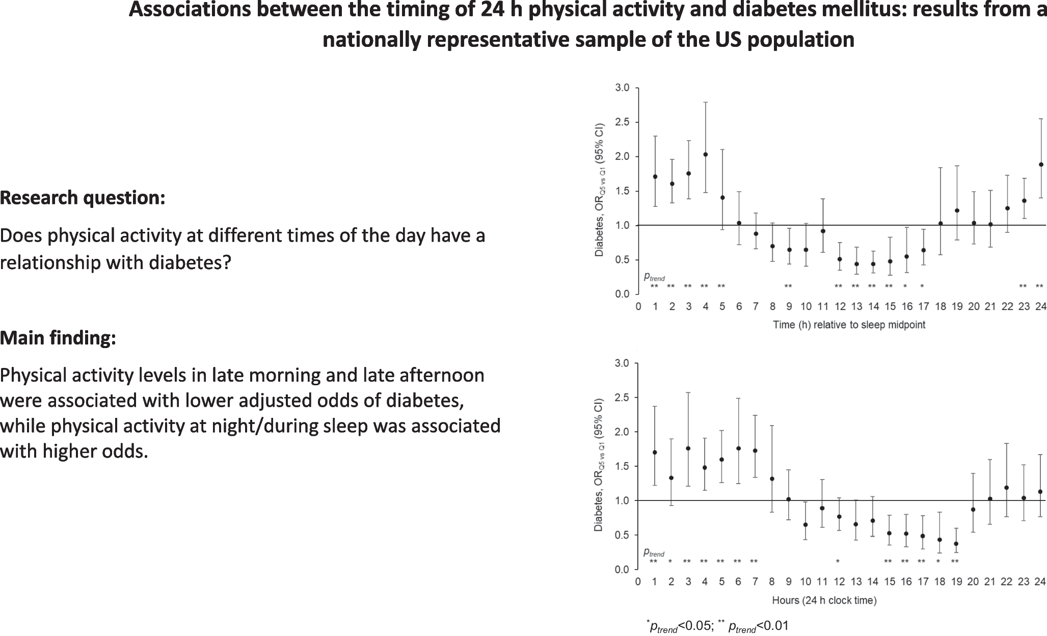
The protocol for the physical activity monitor component in NHANES 2011–2014 is available online [22]. Briefly, participants aged ≥3 years wore a triaxial actigraph device (ActiGraph GT3X+) on the wrist of the non-dominant hand for seven full days (midnight to midnight) to record 24 h movements at a sampling frequency of 80 Hz. Raw data were processed to determine whether signal patterns were unlikely to be caused by human movement, and those determined as such were flagged. Details about data quality and the meaning of flags are published on the NHANES website [23]. Using a published open-source algorithm, John et al harmonised and aggregated raw accelerometry data in NHANES 2011–2014 to generate a monitor-independent movement summary (MIMS) unit, which was optimised to capture normal human motion [24]. Using aggregated data, activity at the minute level was further classified as ‘wake wear’, ‘sleep wear’ or ‘non-wear’ [24]. Using the same criteria as in our previous studies [25,26,27], we defined a valid minute as one labelled as wake or sleep, and a valid day as one having at least 20 h of valid data. This classification was used to exclude participants with insufficient data (as indicated above). To measure total activity levels for each hour, we used the minute-level MIMS data because this measure was commonly used in epidemiological studies to examine physical activity patterns and their relationships with various health outcomes in the USA [3, 28, 29]. We calculated the mean of minute-level MIMS units for each hourly window defined by two methods: (1) relative to the average sleep midpoint of each individual (e.g. 0–59 min after the midpoint, primary method; see below for sleep midpoint calculation); and (2) based on clock time (e.g. 00:01–01:00 hours, secondary method).

To calculate the average sleep midpoint, we first determined the average time of sleep onset and offset for each individual. For this calculation, we focused on sleep time between the period of 20:00–10:00 hours to minimise the influence of unusual/extreme sleep windows that may be severely misaligned with the circadian clock. To determine the sleep onset time, we calculated the percentage of sleep wear time within a rolling 30 min window, starting from 20:00 hours, and defined sleep onset as the first minute labelled as sleep wear within the first rolling window during which the sleep wear time was 15 min (50%) or higher. To determine sleep offset, we applied the same process backward, starting from 10:00 hours: the first window was 09:31–10:00 hours, and if there were fewer than 15 min labelled as sleep, the window was rolled 1 min backward to 09:30–09:59 hours. This process continued until 15 or more minutes of sleep time were recorded within a window. The individual’s overall sleep midpoint was then defined as the midpoint between the averaged sleep onset and offset time across the recording period. We further calculated the sleep midpoint on weekends by using sleep onset and offset time between 20:00 hours on Friday and 10:00 hours on Sunday. We used the weekend sleep midpoint as an indicator of chronotype because it is less influenced by work schedule and other external constraints and thus more likely to reflect the individual’s internal propensity to sleep at a certain time of the day.

Diabetes mellitus and glycaemic markers

The primary outcome was diabetes status. Individuals with diabetes mellitus were defined using the following criteria: HbA1c ≥48 mmol/mol (6.5%) as measured using a Tosoh automated glycohaemoglobin analyser HLC-723G8, or self-reported diagnosis. Secondary outcomes included four glycaemic markers (fasting glucose, fasting insulin, HOMA-IR and 2 h OGTT results). Details on laboratory assays for fasting glucose, fasting insulin, HOMA-IR and OGTT and for each survey cycle are published on the NHANES website [30,31,32,33]. We applied the conversion algorithm as recommended by NHANES to match the 2013–2014 fasting insulin values to the 2011–2012 values to account for differences in laboratory protocols between the cycles: insulin2011–2012 =\(10^}_\left[}_\right]-0.0802\right)}\). HOMA-IR was calculated as previously reported [34]. OGTT results were based on plasma glucose levels measured 2 h after ingesting 75 g glucose orally (Trutol glucose solution, Thermo Fisher Scientific). For the OGTT, there were several additional exclusion criteria, including haemophilia and chemotherapy safety exclusions, fasting for less than 9 h, taking insulin or oral medications for diabetes, refusing phlebotomy and not drinking the entire glucose solution within the allotted time. All four secondary outcome variables were loge-transformed to improve normality.

Covariates

The following variables were included as covariates in regression analyses: sociodemographic characteristics and lifestyle factors (age, gender, race/ethnicity, education, household income, marital status, smoking, alcohol consumption; all as reported during home-based interviews), BMI (calculated based on weight and height measured at the NHANES mobile examination centre), total energy intake (estimated based on two 24 h dietary recalls), sleep duration (measured as the daily average of total minutes categorised as sleep wear), and total physical activity (measured as the average of the daily sum of per-minute MIMS values across the recording period).

Statistical analysis

We divided hourly physical activity levels (mean MIMS as described above), defined either based on clock time or relative to the overall sleep midpoint, into quintiles, and used the lowest quintile as the reference group. For each 1 h window, we examined the association between quintiles of physical activity levels and diabetes status using multiple logistic regression, adjusted for age, gender, race/ethnicity, education, household income, marital status, smoking status, alcohol intake, total energy intake, sleep duration, sleep midpoint and total physical activity. For analyses focusing on glycaemic markers, we used multiple linear regression adjusted for the same covariates. p values for trend were determined by modelling quintiles of physical activity variables as continuous (i.e. 1–5 for Q1–Q5). For sensitivity analysis, we excluded participants with extreme sleep duration (≤4 or ≥10 h). We also performed subgroup analyses focusing on the primary outcome (i.e. diabetes) stratified by gender (men/women), age (<65 years/≥65 years), race/ethnicity (non-Hispanic white, non-Hispanic black, Hispanic), chronotype (weekend sleep midpoint before 03:15 (median) vs after 03:15 hours) and sleep duration (<7 h/≥7 h). For subgroup analyses, we modelled quintiles of hourly activity levels as a continuous variable to preserve statistical power, and relied on visualisation of the 24 h patterns of associations to identify potential similarities and differences in a qualitative fashion. To account for the complex, multi-stage probability sampling design of NHANES, we used the following: the full-sample mobile examination centre examination weight for the analysis focusing on diabetes, the fasting sub-sample weight for fasting glucose, fasting insulin and HOMA-IR, and the OGTT sub-sample weight for OGTT results. All analyses were performed using SAS 9.4 (SAS Institute).