Fly work and generation of mutant flies by CRISPR–Cas9 genome engineering

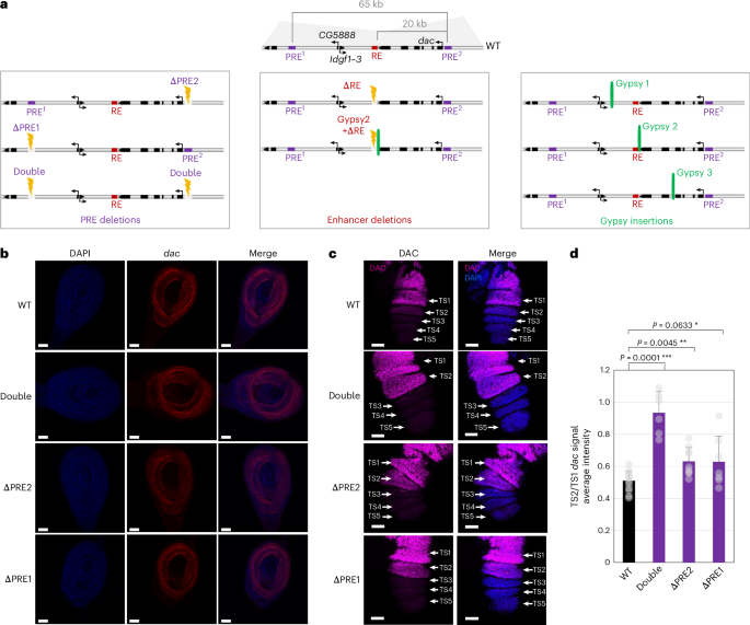
All flies were raised on standard corn meal yeast extract medium at 25 °C. CRISPR–Cas9 mutant fly lines double, ΔPRE1, ΔPRE2 and gypsy 1 were described in a previous study22. Sequences of guide RNAs (gRNAs) used to create fly lines gypsy 2, gypsy 3, ΔRE and gypsy 2 + ΔRE are described in Supplementary Table 2. Sense and antisense oligonucleotides were annealed and phosphorylated by the T4 polynucleotide kinase (New England Biolabs, M0201S) before being inserted inside a pCFD3 plasmid (Addgene, 49410) previously digested by BbsI (NEB, R0539S). To create the pHD-dsRED donor plasmid (Addgene) containing a removable (floxed) 3XP3–dsRED construct flanked by loxP sites and DNA fragments having homology to the target regions (homology arms) serving as a template for homology-directed repair, 1.5-kb genomic DNA fragments were amplified by PCR (Supplementary Table 2) and inserted into the pHD-dsRED plasmid using Gibson assembly (kit NEBuilder; New England Biolabs, E2621S).

The gypsy insulator was amplified from the plasmid (Gy)w(Gy) described in a previous study48 and introduced into the donor plasmid cut by SpeI and BglII using Gibson cloning (Supplementary Table 2). To generate mutant fly lines, gRNA-containing pCFD3 and pHD-dsRED donor plasmids were injected into flies expressing Cas9 in the germline (vas-Cas9(X) RFP−; Bloomington, 55821). Injections and dsRED screening were performed by BestGene (https://www.thebestgene.com/). To remove the dsRED reporter construct, mutant flies were crossed with a fly line expressing CRE recombinase (Bloomington, 34516). To generate the gypsy 2 + ΔRE mutant line, gRNAs targeting the RE and corresponding donor plasmid were injected into gypsy 2 mutant lines previously generated and expressing Cas9 (vas-Cas9(III)). Coordinates and sequences of deleted regions can be found in Supplementary Table 3. Genotypes of mutant fly lines were confirmed by PCR genotyping and sequencing analysis of the mutated region.

Immunostaining experiments

For immunostaining, third-instar imaginal leg discs were dissected at room temperature in sterile Schneider medium. Pupae were selected at the very beginning of pupation, where pupae can be recognized by their white color (a pupal stage that lasts 1 h), and were dissected 3.5–4 h later. The discs were then fixed for 20 min in 4% formaldehyde and were permeabilized for 1 h in PBS + 0.5% Triton (for larval leg discs) or 0.8% Triton (for pupal leg discs). The samples were then incubated for 1 h in 3% BSA PBTr (1× PBS + 0.5% Triton X-100). DAC primary antibody was diluted 1:400 (DSHB mAbdac1-1) in 1% BSA PBTr and incubated overnight at 4 °C on a rotating wheel. The leg discs were washed in PBTr before adding the secondary antibody at 1:1,000 dilution (Thermo Fisher Scientific, A-31571) and incubated for 2 h at room temperature on a rotating wheel. Finally, the discs were extensively washed in PBTr. The proximal segments of the leg discs were removed by dissection to only keep the TSs, which were subsequently mounted on microscope slides using ProLong Gold reagent (Invitrogen, P36930). The different images were acquired on a Zeiss axioimager Z2 Apoptome Leica SP8 confocal microscope using the same settings for all mutant lines and analyzed using Fiji software.

RNA FISH experiments

RNA FISH probes were prepared with an RNA FISH probe kit (Thermo Fisher Scientific, F32956) from DNA probes amplified with the primers described in Supplementary Table 2. Third-instar imaginal leg discs were quickly dissected in Schneider medium. Pupae were selected at the very beginning of pupation, where pupae can be recognized by their white color (a pupal stage that lasts 1 h), and were dissected 3.5–4 h later. The discs were then fixed with 4% formaldehyde before being permeabilized with PBTr for 4 h. Subsequently, discs were incubated for 10 min with 50% PBT (PBS + 1% Triton), 50% hybridization solution (50% formamide, 5× saline–sodium citrate (SSC), 100 g ml−1 fragmented salmon testes DNA, 50 g ml−1 heparin and 0.2% Tween-20) at room temperature. The samples were incubated for 45 min and then 1 h in hybridization solution at 55 °C. In parallel, a previously tested optimal concentration of labeled probe was diluted in 50 µl of hybridization solution, heated for 2 min at 85 °C and chilled on ice to denature RNA secondary structures. The discs were then incubated overnight with 50 µl of probe solution at 55 °C. The day after, the samples were washed three times at 55 °C with hybridization solution and twice with PBT. The proximal segments of the leg discs are removed by dissection to only keep the TSs, which were mounted on microscope slides using ProLong Gold reagent (Invitrogen, P36930). Images were acquired on a Zeiss axioimager Z2 APopoteme Leca SP8 confocal microscope using the same settings for all mutant lines and analyzed using Fiji software.

Hi-C experiments

Hi-C experiments were performed using the EpiTect Hi-C Kit (Qiagen, 59971). All Hi-C experiments were performed in two or three independent experiments using 50 third-instar imaginal leg discs or early pupal discs. Briefly, discs were homogenized and fixed in activated buffer T and 2% formaldehyde using tissue masher tubes (Biomasher II (EOG-sterilized), 320103). Tissue was digested by adding 25 μl of collagenase I and II (40 mg ml−1) for 1 h at 37 °C. Samples were centrifuged and supernatant was carefully aspirated, leaving ~250 μl of solution in the tube. Then, 250 μl of QIAseq beads equilibrated to room temperature were added to bind nuclei to the beads and all subsequent reactions were performed on the beads according to the manufacturer’s protocol. Libraries were sequenced at BGI (https://www.bgi.com/) with 150-bp paired-end reads (approximately 400 million reads per replicate).

Hi-C analysis

Raw data from Hi-C sequencing were processed using the ‘scHiC2’ pipeline. Sequencing statistics are summarized in Supplementary Table 4. Valid interactions were stored in a database using the ‘misha’ R package (https://github.com/msauria/misha-package). Extracting the valid interactions from the misha database, the ‘shaman’ R package (https://bitbucket.org/tanaylab/shaman) was used for computing the Hi-C expected models, Hi-C scores with parameters k = 250 and k_exp = 500 (Figs. 2a, 3c and 4a) and differential Hi-C interaction scores with parameters k = 250 and k_exp = 250, with the compared datasets downsampled to have the same number of valid pairs in chromosome 2L (chr2L) for each comparison (Fig. 4b). Specifically, Hi-C scores quantify the contact enrichment (positive values) or depletion (negative values) of each bin of the map with respect to a statistical model used to evaluate the expected number of counts. To generate this expected model, we randomized the observed Hi-C contacts using a Markov chain Monte Carlo-like approach per chromosome49. Shuffling was conducted such that the marginal coverage and decay of the number of observed contacts with the genomic distance were preserved but any features of genome organization (for example, TADs or loops) were not. These expected maps were generated for each biological replicate separately and contained twice the number of observed cis contacts. Next, the score for each contact in the observed contact matrix was calculated using the k nearest neighbors (kNN) strategy49. In brief, the distributions of two-dimensional Euclidean distances between the observed contact and its nearest k_exp neighbors in the pooled observed and pooled expected (per cell type) data were compared, using Kolmogorov–Smirnov D statistics to visualize positive (higher density in observed data) and negative (lower density in observed data) enrichments. These D scores were then used for visualization (using a scale from −100 to +100) and are referred to as Hi-C scores in the text. Accordingly, the color scale of the Hi-C scores comprises both positive and negative values. When computing the differential Hi-C scores maps of Fig. 4b, the reference dataset was used as the expected model.

For each condition, the Hi-C interaction quantifications at the dac PRE loop (Figs. 2c, 3d and 4e) were performed by considering the Hi-C scores between two regions of 6 kb, chr2L:16419514–16425515 and chr2L:16482929–16488930), including the PRE1 and PRE2, respectively (Supplementary Table 3). The distributions of Hi-C scores (Figs. 2c, 3d and 4e) are represented as box plots showing the median (central line), the 75th and 25th percentiles (box limits) and 1.5 × the interquartile range (IQR; whiskers). Each of the comparisons of the Hi-C interaction quantifications at the dac PRE loop was performed between a reference condition (embryo in Fig. 2c and WT larvae in Figs. 3d and 4e) and each of the other conditions present in the same figure. An unpaired two-sided Wilcoxon statistical test (with the null hypothesis that the true median shift is equal to zero and assuming that the two variables are not normally distributed) was used to estimate the reported P values. The annotation of the Polycomb-associated TADs in chr2L from a previous study5 was used to compute the number of Hi-C interactions within the PcG TAD, which were then normalized by the total number of valid pairs at the corresponding developmental stage (embryo, larvae or pupae). The distributions of these interaction frequencies are shown in the violin and box plots of Fig. 2b as the log2 ratios of embryo over the larval and pupal leg discs. The box plots show the median (central line), the 75th and 25th percentiles (box limits) and 1.5 × IQR (whiskers). An unpaired two-sided Wilcoxon statistical test (with the null hypothesis that the true median shift is equal to zero and assuming that the two variables are not normally distributed) was used to estimate the reported P values. The ISs50 were computed on the observed Hi-C datasets binned at 2-kb resolution with windows of 100, 150, 200, 250 and 300 kb, resulting in five values per bin, and were stored in the misha database using an in-house R script. The mean and s.d. for each of the 2-kb bins were computed for the plots in Figs. 3e and 4c. The quantification of the ISs at gypsy insertions and R0–R12 regions was performed by applying a pairwise statistical comparison of the five IS quantifications per 2-kb bin. The P values in Fig. 4d and Extended Data Fig. 4b resulted from a Welch t-test (with the null hypothesis that the true difference in means is equal to zero and assuming that the variances of the samples are not equal) between the WT condition and each of the gypsy mutants at the corresponding locus. All plots of Hi-C maps (Figs. 2a, 3c and 4a,b), Hi-C interaction score comparisons (Figs. 2c, 3d and 4e), IS profiles (Figs. 3e and 4c) and P values of IS comparisons (Fig. 4d) were obtained with in-house R scripts.

Hi-M library preparation

The oligopaint library covering the dac region consists of 52-mer sequences with genome homology ordered from CustomArray. These sequences were obtained from the oligopaint public database (http://genetics.med.harvard.edu/oligopaints). From the initial design of the library, we selected 20-mers with an average probe density of 9–17 probes per kb. Each barcode contained 45 probes covering 3.8 kb on average (Supplementary Table 1). Each oligo was composed of five different regions: (1) a 21-nt forward universal priming region for library amplification; (2) two 20-nt readout regions separated by an A for barcoding; (3) a 42-nt genome homology region; (4) a duplication of one 20-nt readout region; and (5) a 21-nt reverse universal priming region.

The procedure for oligopaint library amplification was previously described26,42,51,52. It consists of seven steps: (1) an emulsion PCR (emPCR) to extract the dac library from the oligonucleotide pool using universal primers; (2) a limited-cycle PCR performed on the emPCR to identify the most efficient amplification cycle; (3) a large-scale PCR with a T7 promoter on the reverse primer; (4) an in vitro T7 transcription; (5) RT to transform RNAs into single-stranded DNA (ssDNA); (6) an alkaline hydrolysis for the removal of the intermediate RNA; and (7) ssDNA purification and concentration.

Each barcode is unique and specific to an adaptor oligo. The adaptor oligo serves as a bridge between the readout region and an Alexa Fluor 647-labeled secondary oligonucleotide. The fluorescently labeled part of the secondary probe is attached by a disulfide leakage that can be cleaved (chemical bleaching) during the sequential imaging of FISH probes51. For the fiducial, we used an adaptor oligo complementary to the reverse primer of the library and specific to a secondary probe bound to a noncleavable rhodamine red fluorophore. Adaptors and fluorescently labeled secondary probes were synthesized and purchased from Integrated DNA Technologies.

Hi-M library hybridization

Pupae were collected at the beginning of pupation (white pupae) and dissected 3.5–4 h later. The dissected leg disc were fixed with 4% formaldehyde before being permeabilized with PBTr for 4 h. The discs were then progressively washed in four different concentrations of Triton and pHM (2× SSC and 0.1 M NaH2PO4 pH 7; 20%, 50%, 80% and 100%) for 20 min in each buffer at room temperature on a rotating wheel. Then, the discs were incubated overnight in 225 pmol of the library diluted in 30 µl of FISH hybridization buffer (FHB; 50% formamide, 2× SSC, 0.5 mg ml−1 salmon sperm DNA and 10% dextran sulfate). The probes and the discs in pHM were heated at 80 °C. The incubation of the leg discs in the FHB + probe buffer was performed in a PCR machine from 80 °C to 37 °C with a temperature decrease of 1 °C every 10 min. The next day, discs were washed two times with 50% formamide, 2× SSC and 0.3% CHAPS and sequentially washed with four different concentrations of formamide and PBT (40%, 30%, 20% and 10% formamide) for 20 min per buffer on a rotating wheel. Finally, the discs were washed with PBT, fixed with 4% formaldehyde in PBS, washed with PBS and stored at 4 °C.

Hi-M imaging system

Hi-M experiments were performed with a homemade wide-field and epifluorescence microscope. This setup includes a rapid automated modular microscope (Applied Scientific Instrumentation) coupled with a microfluidic device as previously described26,42. The microscope and fluidics system were controlled using Qudi-HiM (our homemade hardware control package)53. The fluidics system permitted the automated and sequential hybridizations of the probes. The solutions were delivered to the sample by a combination of three eight-way valves (HVXM 8-5, Hamilton), a negative pressure pump (MFCS-EZ, Fluigent) and an FCS2 flow chamber (Bioptechs). The excitation was performed by three different lasers: 405 nm (Obis 405, 100 mW; Coherent), 561 nm (Sapphire 561 LP, 150 mW; Coherent) and 642 nm (VFL-0-1000-642-OEM1, 1 W; MPB communications). The fluorescence was collected through a Nikon APO ×60 (1.2 numerical aperture) water-immersion objective lens mounted on a closed-loop piezoelectric stage (Nano-F100, Mad City Labs). Images were acquired using a scientific complementary metal–oxide–semiconductor camera (ORCA Flash 4.0 V3, Hamamatsu) with an effective optical pixel size of 106 nm. To correct axial drift in real time, we used a homemade autofocus system composed of a 785-nm laser (OBIS 785, 100 mW; Coherent) and an infrared-sensitive camera (DCC1545M, Thorlabs).

Acquisition of Hi-M datasets

The proximal part of the pupal leg discs was removed by dissection to only keep the TSs. About 15–20 TSs were aligned on a 2% agar–PBS pad and then attached onto a 40-mm round coverslip previously functionalized with trimethoxysilane and 10% poly(l-lysine). The slide was then mounted onto the flow chamber. Pupal leg discs were first incubated with the fiducial adaptor (25 nM of the adaptor specific to the reverse primer, 2× SSC and 40% v/v formamide) for 20 min and then washed with a washing buffer solution (2× SSC and 40% v/v formamide) for 10 min. To complete the hybridization of the fiducial, we did a second round of incubation with the appropriate secondary oligo (25 nM of rhodamine-red-labeled probe, 2× SSC and 40% v/v formamide) for 20 min and washed again for 10 min with the washing buffer solution. After a 5-min wash with 2× SSC, we proceeded with nuclear staining with 0.5 µg ml−1 of DAPI in PBS for 20 min. After another 5-min wash with 2× SSC, the imaging buffer (1× PBS, 5% glucose, 0.5 mg ml−1 glucose oxidase and 0.05 mg ml−1 catalase) was injected to limit fiducial photobleaching during the acquisition. An image stack (200 µm × 200 µm region of interest) was acquired for each of the 10–15 pupal leg discs. The DAPI and the fiducial were sequentially imaged (using 405-nm and 561-nm lasers) with a z step size of 250 nm for a total range of 17.5 µm.

Next, adaptor oligos and the secondary probe were sequentially hybridized, acquired and photobleached to image the whole dac oligopaint library. The following steps were performed for each of the 22 barcodes: (1) adaptor (40 nM of adaptor oligonucleotide, 2× SSC and 40% v/v formamide) injection and incubation for 10 min; (2) imaging probe (40 nM secondary probe, 2× SSC and 40% v/v formamide) injection and incubation for 10 min; (3) 10-min wash with washing buffer solution; (4) 5-min wash with 2× SSC; (5) imaging buffer injection and sequential acquisition of fiducial and barcode with 561-nm and 642-nm lasers; (6) chemical bleaching (2× SCC and 50 mM TCEP) of the imaging probe; and (7) 5-min wash with 2× SSC before a new cycle of hybridization.

Image processing and Hi-M analysis

Raw TIFF images were deconvolved using Huygens Professional 21.04 (Scientific Volume Imaging, https://svi.nl). Hi-M analysis was performed using pyHiM, a homemade analysis pipeline (https://pyhim.readthedocs.io/en/latest/)54, as previously described55. First, images were z-projected by applying either the sum for DAPI channels or the maximum intensity for the barcodes and fiducial. For each cycle of hybridization, fiducial images were used to register the corresponding barcode image using global and local registration methods. Barcodes and fiducials were segmented in 3D using a neural network, followed by 3D localization of the center of each barcode mask54. The fiducial oligo bound to the universal priming regions, thus labeling the entire dac locus. Therefore, we built chromatin traces by combining the DNA FISH spots colocalizing within single fiducial masks. DAPI images were used to manually segment the different TSs (TS1, TS2, TS3, TS4 or TS5). Pairwise distance (PWD) matrices were calculated for each single chromatin trace. From a list of PWD maps, we calculated the proximity frequencies as the number of chromatin traces in which PWDs were within 250 nm, normalized by the number of chromatin traces containing both barcodes. Hi-M maps of the WT condition were generated from 51,622 total traces from 48 pupal leg discs from two independent biological replicates. Hi-M maps of the Gypsy 2 mutant were produced from 63,458 total traces of 51 pupal leg discs from two independent biological replicates. Hi-M matrices were generated for all the TSs combined (TS1, TS2, TS3, TS4 and TS5), as well as for TS1, TS2 and TS3 + TS4. Each trace contained at least 12% of the barcodes. Virtual 4C figures were obtained by plotting the PWDs between the anchored barcode or viewpoint with the remainder of the barcodes of an Hi-M matrix.

Wilcoxon two-sided rank tests between the PWD distributions of the barcodes containing the RE and the dac promoter were performed to test the hypothesis that two independent samples (for example, WT and gypsy mutant) were drawn from the same distribution. P values < 0.05 were considered significant to reject the hypothesis (that is, a 5% significance level).

We estimated the error in the measurement of the median RE–dac promoter distance by performing bootstrapping analysis. For this, we performed 1,000 bootstrapping cycles drawn from the experimental distribution of PWDs to estimate the s.d. in the determination of the median distance. The errors were between 8 and 25 nm for the WT condition.

4C-seq experiments

For 4C, either about 3,000 embryos were collected or 300 third-instar imaginal leg discs were dissected, homogenized and fixed in 2% formaldehyde diluted in nuclear permeabilization (NP) buffer (15 mM HEPES pH 7.6, 60 mM KCl, 15 mM NaCl, 4 mM MgCl2, 0.1% Triton X-100, 0.5 mM DTT and 1× protease inhibitors (complete EDTA-free tablets; Roche, 11 873 580 001)) for 10 min at room temperature. Fixation was stopped by adding 2 M glycine for 5 min. The samples were then washed once in NP buffer and twice in 1.25× NEB3 buffer and the pellet of fixed cells was frozen in liquid nitrogen and conserved at −80 °C.

The chromatin pellet was then layered with 500 μl of 1.25× DpnII buffer without resuspension and centrifuged. The pellet was resuspended in 250 μl of 1.25× DpnII buffer. Then, 10 μl of 10% SDS was added and incubated for 20 min at 65 °C and 40 min at 37 °C. Chromatin was then split into 250-μl 1.25× DpnII buffer aliquots of 5–6 × 106 cells and incubated for 1 h at 37 °C with 3.3% Triton X (final concentration). Samples were digested with 500 units of DpnII overnight. The day after, DpnII enzyme was inactivated by heating the samples at 65 °C for 20 min. The fragments were then ligated for 5 h at 16 °C with T4 ligase (2,000 units per µl) and digested overnight with proteinase K at 65 °C. The day after, RNA was degraded by RNAse A solution for 1 h at 37 °C. DNA was purified with Ampure beads without size selection and digested overnight with NlaIII enzyme. The next day, the DNA fragments were circularized by overnight ligation with T4 ligase (2,000 units per µl) in a large buffer volume. Next, circularized DNA was purified by Ampure beads without size selection. Lastly, 4C PCR was performed with the primers described in Supplementary Table 2. The amplified DNA was purified with Ampure beads. The sequencing libraries were produced with an Illumina kit (Illumina, 20015964). Sequencing (paired-end sequencing with 150-bp reads; approximately 4 Gb per sample) was performed by Novogene (https://en.novogene.com/).

4C-seq processing and analysis

Using a custom-made python script, FASTQ sequencing files were split using 4C primer sequences to obtain individual FASTQ files only containing reads from a single viewpoint per genotype and tissue type. Accordingly, the reads were trimmed to remove viewpoint sequences up to the restriction sites. Subsequently, the trimmed reads were aligned against the DM6 reference assembly using Bowtie56 with the parameters ‘-a -v 0 -m 1’ (no mismatches and no multiple alignments allowed). The number of successfully aligned reads can be found in Supplementary Table 5. The aligned reads were mapped to restriction fragments and genomic bins of 1 kb using HiCdat57 to obtain tabular files describing the number of reads (that is, contact frequencies) for a given fragment or genomic bin. All subsequent analysis steps were conducted using R. Depending on the 4C samples genotypes and viewpoints, contact frequencies arising from the viewpoint (±4 bins) and contact frequencies mapping to genotype-specific deletions were masked by setting them to zero (Supplementary Table 3). Then, data from individual samples were normalized for differing overall library size (counts per million).

To analyze differences between different genotypes, t-tests using triplicate data per genotype were performed for each 1-kb genomic bin along the region of interest (chr2L:1630000–16600000). No multiple-testing correction was performed. Subsequently, the differences of the average of triplicates were plotted and genomic bins that exhibited P values < 0.1 were highlighted.

qRT–PCR experiments

Embryos were collected in a 16–20-h developmental time window. Third-instar imaginal leg discs or early pupal leg discs (3.5–4 hs after pupation) were quickly dissected (<30 min) in Schneider medium and transferred into Trizol. RNA was extracted using Trizol reagent and purified using an RNA clean and concentrator kit (Zymo Research, R1015) following the instructions and using DNAse I (Qiagen, 79254). Then, 250 ng of purified RNA was used for RT using the Maxima first-strand complementary DNA synthesis kit for RT–qPCR with dsDNase (Thermo Fisher Scientific, K1671) following the manufacturer’s recommendations. Finally, quantification of the RT product was performed on a LightCycler 480 (Roche) with the primers listed in Supplementary Table 2. Data analysis was performed on LightCycler software. Expression levels were normalized to the housekeeping gene RP49.

qCHIP experiments

qChIP experiments were performed as described in a previous study58 with minor modifications. Chromatin was sonicated using a Bioruptor Pico (Diagenode) for 7 min (30 s on, 30 s off). Su(HW) antibody was diluted 1:100 for the immunoprecipitation. After decrosslinking, DNA was purified using MicroChIP DiaPure columns from Diagenode. Enrichment of DNA fragments was analyzed using a real-time PCR LightCycler 480 (Roche). The primers used are indicated in Supplementary Table 2.

CUT&RUN experiments

CUT&RUN experiments were performed as described in the literature59 with minor modifications. A total of 50 eye discs were dissected in Schneider medium, centrifuged for 3 min at 700g and washed twice with Wash+ buffer before the addition of concanavalin A-coated beads. MNase digestion (pAG-MNase Enzyme from Cell Signaling) was performed for 30 min on ice. After proteinase K digestion, DNA was recovered using SPRIselect beads and eluted in 50 μl of Tris-EDTA. DNA libraries for sequencing were prepared using the NEBNext Ultra II DNA library prep kit for Illumina. Sequencing (paired-end sequencing with 150-bp reads; approximately 2 Gb per sample) was performed by Novogene (https://en.novogene.com/). H3K27me3 antibody (Active Motif, 39155) was diluted 1:100. IgG antibody (1:100, Cell Signaling Technology, 2729S) was used as a control.

CUT&RUN analysis

The quality of the reads was assessed using FastQC. FASTQ files were aligned to the D. melanogaster reference genome dm6 using Bowtie 2 (version 2.4.2)60 with the following parameters: ‘--local --very-sensitive-local --no-unal --no-mixed --no-discordant --phred33 -I 10 -X 700’. SAM files were compressed into BAM files using SAMtools (version 1.16.1) and reads with low mapping quality (Phred score < 30) were discarded. Duplicate reads were removed using Sambamba markdup (version 1.0.0)61 with the following parameters: ‘-r --hash-table-size 500000 --overflow-list-size 500000’. For visualization, replicates were merged using SAMtools ‘merge’ with default parameters and reads per kilobase per million mapped reads (RPKM)-normalized bigWig binary files were generated using the bamCoverage (version 3.5.5) function from deepTools2 (ref. 62) with the following parameters: ‘--normalizeUsing RPKM --ignoreDuplicates -e 0 -bs 10’. Genome browser plots were generated using the pyGenomeTracks package (version 3.8)63. The 131 Drosophila Polycomb domains22 were used for differential enrichment analysis using the DESeq2 method from the ‘DiffBind’ R package (version 3.12.0). Differential quantification results of H3K27me3 levels within Polycomb domains are summarized in Supplementary Table 6.

Reporting summary

Further information on research design is available in the Nature Portfolio Reporting Summary linked to this article.