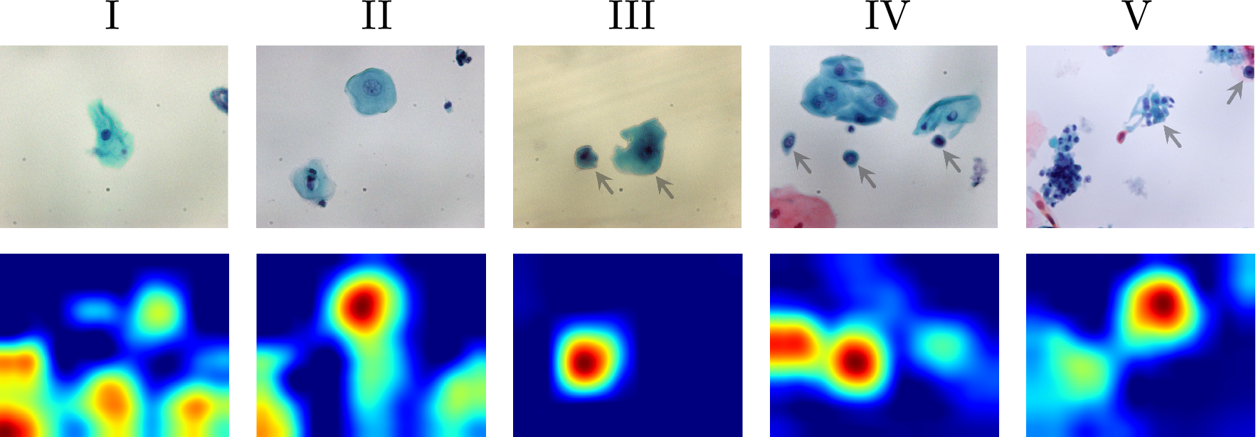
Examples of background removal test results on oral cytology images. The first row presents original images of Pap classes I to V. Our model predicts the foreground cells as the background removal results. Since the cells are darker than the background, their pixel values are negative in the prediction. To display the results as shown in the second row, we adjusted the predicted images by adding a uniform imaginary background of 0.8

We assessed the background removal of the Pap-stained cell images. The image dataset consisted of \(5,\!041\) oral cytology images collected from 31 subjects at the Nagasaki University Hospital, as illustrated in Fig. 1. All color images were resized from \(1,\!280\times 1,\!024\) to \(320\times 256\) (\(c=3\), \(m=81,\!920\)), and their pixel values were normalized to the range [0, 1]. We used twenty subjects to form a training dataset, six subjects for validation, and the remaining five subjects for testing. To train our model shown in Fig. 2 with the loss function in Eq. (1), we set the hyperparameters \(\lambda =1/\sqrt\approx 3.49\times 10^\) and \(\lambda _}=5.0\times 10^\) and ran the Adam optimizer with a mini-batch size \(n=32\) and a learning rate \(\alpha =1.0\times 10^\) for 30 epochs. The background removal results for the validation images were insensitive to hyperparameters around these values. We observed stable convergence to the well-generalized model in this setting: the training loss almost monotonically decreased, and the validation loss did not tend to increase.

Figure 3 shows examples of the input and output of the model for the test images. Our model successfully predicted the foreground cells with the background removed in almost all the test images unless, as in the Pap class III example, the microscopic slide was heavily deteriorated. The small black spots isolated in the background are debris. Despite their sparsity, most of them were removed as well. This can be attributed to the total variation that makes the model learn to reject isolated pixels. As a side effect of the total variation, the predicted cells were slightly blurred.

Distribution of class discriminative features with and without background removal. The first row shows an example of test image for each Pap class. The corresponding Grad-CAMs in the second row were obtained from a transfer learning classifier for the test images with background removed. The classifier was fine-tuned on oral cytology images with background removed. The first and third rows are the same as the first and second rows in Fig. 1

We confirmed the effectiveness of our background removal method in debiasing cell classification. We built an image classifier in the manner of transfer learning. We utilized the feature extractor of VGG16 [25], pre-trained on ImageNet [6], as the backbone of the classifier. A fully connected layer was attached to classify whether a cytology image was of normal (Pap class I or II) or abnormal (Pap class III or above) based on the global average pooling (GAP) [15] over 512 feature maps from the backbone. We trained a background removal model as described in the previous section and fine-tuned the classifier on the foreground cell images predicted by this model. We minimized the cross-entropy loss between the classifier outputs and the normal/abnormal labels using the Adam optimizer with a learning rate of \(10^\) until the validation accuracy stabilized. For comparison, we also built an image classifier that was fine-tuned in the same manner as the original training images without using the background removal model.

We tested two image classifiers, one with background removal and one without, on test images. We present examples of Grad-CAMs [24] for each of the second and third rows of Fig. 4, respectively. Grad-CAMs highlight image features based on the inference of a classifier. The background-removed image classifier mainly focuses on the cells in all test image classes. Some of the expert-annotated cells of interest could be identified for the test images in Pap classes III–V (e.g., the cells indicated by arrows in Fig. 4). On the other hand, the classifier without background removal tended to infer on the basis of the background features for the test images of classes I and II in particular. It is difficult to find evidential features from cells to identify the cytology images of classes I and II as normal, compared to the images in classes III–V containing unique abnormal cells. It can be said that background removal hinders the extraction of discriminative features from patterns of background or debris that correlate with the subject.

We measured the performance of the two classifiers in identifying normal and abnormal cases by conducting repeated random subsampling ten times. The test accuracies with and without background removal were \(76\%\pm 3\%\) and \(81\%\pm 2\%\), respectively. These scores indicate that overestimation was corrected by addressing the background-bias issue, which is further explored in the Discussion section.

We extended the evaluation of our background removal approach in the context of a semantic segmentation task of cells. If our model can accurately subtract backgrounds from cytology images, only the foreground cells should remain. Therefore, we conducted quantitative evaluation of our model’s segmentation quality, utilizing an open dataset for cervical cell segmentation. We proved the superiority of our approach to supervised one and RPCA and assessed the effect of total variation.

We evaluated the proposed semantic segmentation using the ISBI 2014 dataset [16, 17]. The ISBI 2014 dataset is intended as a benchmark for cell detection in cervical cancer cytology. The dataset consists of 135 synthetic grayscale cytology images of size \(512\times 512\) (\(c=1\), \(m=512\times 512=262,\!144\)) with segmentation annotation. We used only 45 images for training and validation purposes, whereas the remaining 90 images were used for testing according to the setup of the dataset. We evaluated our model ten times by cross-validation with repeated random subsampling, where \(n=36\) out of 45 images were randomly selected for training each time. We normalized all pixel values to be in the range [0, 1] by simply dividing them by 255.

The hyperparameters including the binarization threshold were determined by Optuna [1] to maximize the Dice similarity coefficient (DSC) [7, 17] for the validation images. We found \(\lambda \approx 1.14\times 10^\), \(\lambda _}\approx 4.74\times 10^\), and the learning rate \(\alpha =7.22\times 10^\) for the Adam optimizer [14]. The best binarization threshold was \(6.9\times 10^\), which is much smaller than 1/255. We selected the best model for each round of cross-validation using the DSC.

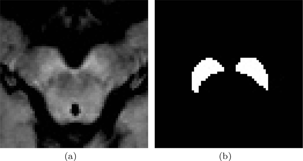
Examples of test images for semantic segmentation and corresponding ground truths in the ISBI 2014 dataset. Cells are sparse in the first and second examples, while they are nonsparse in the third example

Examples of segmentation test results corresponding to the test images shown in Fig. 5. Output with TV shows the predicted foreground cells by our model, while the output without TV shows those by a dual-frame U-Net model trained without total variation for an ablation study. The output of RPCA shows absolute pixel values of sparse components, \(\mathcal \), computed by RPCA. The segmentation results are obtained by binarization of the outputs. The percentages indicate the Dice similarity coefficient (DSC)

Examples of the test images are shown in Fig. 5, and the corresponding model outputs are shown in the first and second rows of Fig. 6. The model successfully separated cells from the background. The binarization detects the cell regions with a mean DSC of \(95.2\%\pm 5.5\%\) (mean ± standard deviation), which outperforms the algorithms presented in [17] and evaluated on the same ISBI 2014 dataset.

The segmentation performance was compared with that of a supervised model. We trained a dual-frame U-Net model with the same architecture as that in our model using the binary cross-entropy loss between its outputs and ground truths. The mean DSC of this supervised model for the test images was \(58\%\pm 31\%\), which suggests overfitting to a small number of training images. We can conclude that our method offers a generalized model without supervision, even for small datasets.

To evaluate the effectiveness of training with the total variation, we conducted an ablation study. We set \(\lambda _}=0\) and revised the hyperparameters by Optuna as \(\lambda \approx 1.05\times 10^\) and \(\alpha =8.49\times 10^\). The best binarization threshold, \(1.8\times 10^\), was much larger than 1/255, indicating a degradation in the ability to distinguish cells with nonzero pixels from the background.

The results of the cell separation and segmentation are presented in the third and fourth rows in Fig. 6. Some low-contrast parts of cytoplasm were missing or fragmented into tiny pieces. Incorporating the total variation in training was confirmed to encourage the formation of cell regions with connected pixels. Without the inclusion of the total variation, the mean DSC for the test images ranged between \(74\% \pm 30\%\). Notably, the performance of the model was highly dependent on how the training data were split in the cross-validation. The total variation was found to stabilize the training, particularly in situations with limited data.

We compared our model with RPCA [4]. All 135 images in the ISBI 2014 dataset were reshaped into a single matrix \(\textbf \in \mathbb ^\). We employed the RPCA algorithm [10, 29] to minimize the objective function in Eq. (3) on the basis of the alternating directions method of multipliers (ADMM) [3, 9]. We implemented it using PyTorch [22] with double precision for fair comparison and numerical stability reasons. We have observed in preliminary experiments that the algorithm converges well within a thousand iterations. The optimal hyperparameter \(\lambda \) was determined to be \(\lambda \approx 1.1\times 10^\) using Optuna [1]. Optuna also found that the best binarization threshold was \(4.8\times 10^\), significantly larger than that of our model.

The results of cell separation and segmentation by RPCA are presented in the last two rows of Fig. 6. RPCA failed to detect the cytoplasm of cells located around the center of the image and incorrectly detected background noise as foreground cells. Since most images in the ISBI 2014 dataset contained one or more cells in their center, portions of them were separated by RPCA into the low-rank backgrounds. The background noise was not of low rank; thus, it was identified as an outlier from plain background. Nonsparse cells, as in the third example, were almost detectable when RPCA was applied to the image of nonsparse cells along with sparse cell images. RPCA scored \(71.9\%\) DSC for the test images, which was outperformed by our model thanks to the TV-sparse foreground feature learning with U-Net.

Comparison of GAP features distributions of oral cytology images with their original backgrounds (left) and backgrounds removed (right). The GAP feature vectors were obtained via a pre-trained VGG16 backbone and visualized by t-SNE. Each point corresponds to a cytology image, and the color represents the Pap smear class

Our model also outperformed RPCA in terms of computational efficiency. Our model can remove backgrounds from approximately 306 images per second at simple precision and 27 images per second at double precision using an A6000 GPU. Our model requires only one forward computation to process each test image, which is significantly faster compared to the iterative process involving singular value decomposition in RPCA until convergence. RPCA took \(252\pm 2.3\) seconds to process 135 images, or approximately two seconds per image using the same GPU.