The study was approved by the institutional review board, and informed consent was obtained by giving patients the opportunity to opt out of the study on the university’s website. Since we started using CT-based navigation for RAO in 2011, 137 navigated RAOs have been performed. The new method was applied to 20 cases with a minimum follow-up period of 1 year until now; therefore, we extracted 20 cases treated with the previous method as controls using propensity score matching for the preoperative Harris Hip Score (HHS), CE angle, AHI, and acetabular roof obliquity (ARO) to compare the accuracy of the new method with that of the previous method.

During preoperative planning, Digital Imaging and Communication in Medicine (DICOM) data of the hip CT scans were converted into a 3D model using a dedicated software (Zed Hip, LEXI, Japan) to create an osteotomy model. The osteotomy model was converted into a Standard Triangulated Language (STL) file using Geomagic Freeform (3D System Corporation, Rock Hill, SC, USA) and was imported into OrthoMap. For preoperative planning, a spherical osteotomy line was envisaged for the acetabulum such that the osteotomy line passed approximately 25 mm proximal to the upper acetabular margin, from the innominate groove of the ischium to the midpoint between the greater sciatic notch and posterior acetabular margin, with the center of the sphere located near the center of the femoral head (or center of the hip joint). The line was planned such that it ran distal to the anterior inferior iliac spine to the center of the pubis and slightly through the iliac inner cortex to avoid cutting into the joint. The diameter of the sphere was generally 80–90 mm and differed among cases.

The amount of rotation of the acetabular fragment after osteotomy was planned until the ARO was 0° in the mid-frontal plane, and the anterior CE angle was 45–50 degrees. The position of the femoral head was planned so that the distance between the center of the femoral head and the Koehler line was 35–40 mm. These values were slightly modified according to the morphology of the patient.

During surgery, the osteotomy line was marked on the lateral side of the ilium using navigation imaging guidance in line with the preoperative plan. The tip of the curved chisel was then registered, and pelvic osteotomy was performed while checking the position of curved chisel tip in real time. After osteotomy, the free fragment was rotated anterolaterally, and absorbable screws were used to fix the rotational fragment.

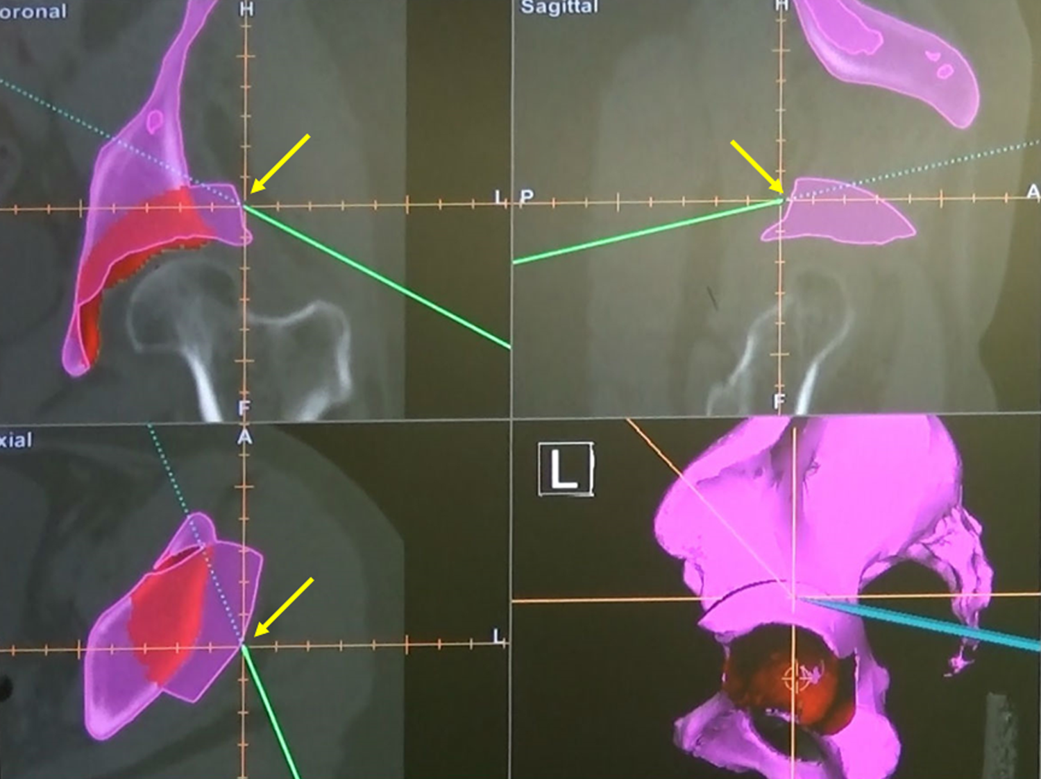
Before the introduction of the new method, the lateral aspect of the rotational fragment was verified after rotation of the bony fragment using navigation to confirm that it was in the preoperative planned position, as described in our previous study [10] (Fig. 1).

Confirmation of the position of the bone fragment after transposition in the previous method. To confirm whether or not the position fits the surface of the planned position after rotation in the preoperative plan, the surface of the rotated bone fragment was touched with a pointer (green bar) after rotation. The yellow arrows show the pointer tip, which touches the surface of the rotated bone fragment at the same position as in the preoperative plan (purple portion)

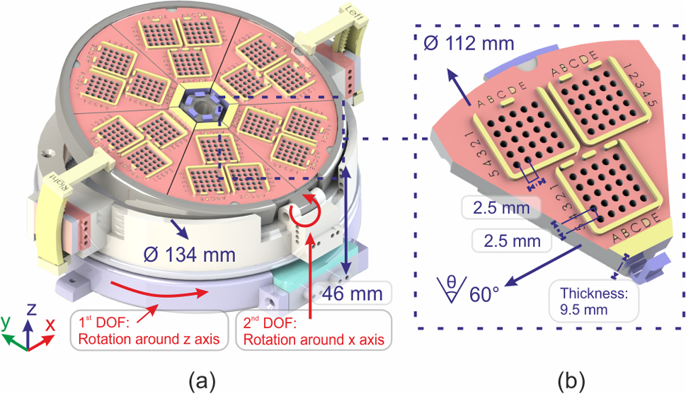
In the new method, an additional step was implemented to create four 2 mm diameter notches (fiducials) around the acetabulum in the preoperative 3D model (Fig. 2a). Thereafter, virtual osteotomy was performed to create a planning model that contained the above-mentioned fiducials. Four fiducials were relocated with the movement of the bony fragments after virtual osteotomy. The relocated position of fiducial #1 was defined as #5, and similarly, fiducial #2 was defined as #6, fiducial #3 as #7, and fiducial #4 as #8 (Fig. 2b). Intraoperatively, these four fiducials were created around the acetabular rim using a high-speed bur under navigation assistance before osteotomy. The fragment position was confirmed using these fiducials, and reorientation was performed by confirming that all four fiducials matched the corresponding relocation points (Fig. 2c, d).

Fiducial point method. a Making four fiducials on the planning model. In the preoperative plan, four 2 mm diameter notches (fiducials: #1–4, blue arrows) are made around the acetabulum in the preoperative planning model before virtual osteotomy. b Relocation of fiducials following vertical osteotomy. Four fiducials are relocated with the movement of bone fragments in the virtually osteotomized planning model. The relocated position of #1 that moves after rotation is defined as #5. Similarly, #2 is defined as #6, #3 as #7, and #4 as #8 after rotation. c Confirmation of position after transposition of the bone fragment with fiducials. Intraoperatively, the fragment position is confirmed using four fiducials and reorientation is performed by confirming that all four fiducials match the relocation corresponding points. Fiducial #2 moves to its corresponding point (#6) after transposition and the bone fragment is fixed with absorbable screws. d Intraoperative confirmation of the position of the fiducials on a computer screen. This figure shows the computer screen during procedure described in (c). On the computer screen, it is confirmed that the tip of the pointer has touched point #6, the point corresponding to #2

The 20 joints in which reorientation was confirmed by tracing the lateral aspect of the rotated fragment with navigation were designated as the “previous method” group, and the 20 hips which were subjected to the new method were designated as the fiducial point method group.

Table 1 shows the patients’ demographic data and preoperative radiographic measurements. No significant differences were found between the two groups due to propensity matching. The primary endpoint of this study was to evaluate whether there was a difference in the preoperative planned and postoperative measured angles between the two groups. The secondary radiological endpoints were the postoperative CE angle, AHI, and ARO, and the clinical endpoint was the HHS at 1 year postoperatively.

CT images of the hip joints acquired preoperatively and at 1 week postoperatively were used for image analysis. A Sensation 16® (Siemens, Munich, Bavaria Germany) CT scanner was used, and the slice thickness was 1.5 mm. Preoperative CT images of the pelvis were loaded onto 3D Slicer (www.slicer.org/) [15], and a 3D model was created by segmenting the pelvis and proximal femur (preoperative model). Based on the preoperative model, virtual RAO was performed on a computer and a model was created for intraoperative navigation (planning model). This planning model was used to perform the RAO. CT was performed again at 1 week postoperatively, and a 3D model of the pelvis and proximal femur was created from the CT images using the same procedure as that before surgery (postoperative model).

The preoperative planned and postoperative measured angles were evaluated using the following two OSSs: a 3D slicer was used to reconstruct the pelvis model from the CT image data, to superimpose the DICOM data and 3D models, and to reconstruct radial section images from normal axial images. CloudCompare 2.6.3 software (www.cloudcompare.org) [16] was then used to calculate the femoral head center position or to register the pre- and post-3D model of the pelvis. The flowchart of image analysis is shown in Fig. 3. First, a 3D model of the pelvis and proximal femur was created based on CT images obtained before and after surgery (Fig. 3a). Next, the preoperative and postoperative image data were registered. The coordinate system used for the measurement was set up using CloudCompare (Fig. 3b). Finally, the registered model was superimposed onto the CT images to perform the measurements (Fig. 3c).

Use of the model-based registration method to compare the preoperative planned and postoperative models. a A three-dimensional (3D) model of the pelvis and proximal femur is created based on the computed tomography (CT) images obtained before and after surgery. b First, each imported model maintains the location within the 3D coordinate system of the original CT data. The antero-pelvic plane was represented as an X–Y plane, and the line passing through the bilateral center of the femoral heads was denoted as the X-axis, while the axis vertical to X–Y plane passing through the femoral head of operative side was denoted as the Z-axis. The planned model is superimposed over the postoperative model using the iterative closest point (ICP) registration function implemented in CloudCompare. c Registered models, which had been registered to the location of the postoperative model, were imported to a stack of postoperative CT images using 3D Slicer; this software enables the display of the cross section of the pelvis in any plane

The planning and postoperative models were loaded into CloudCompare and displayed at different positions in the 3D space, reflecting the position of the pelvis at the time of the CT scan. To accurately superimpose the planning and postoperative models, registration using the iterative closest point algorithm for CloudCompare was used. The planning and postoperative models were moved, and when the mean-squared error of the points that made up each model was 1.0E−5 or less, the planning and postoperative models were considered to exhibit complete superimposition.

After the 3D models were superimposed, the planning model was saved in STL format and imported into 3D Slicer simultaneously with the postoperative CT image. The planning model was displayed at the position of the pelvis on the postoperative CT image. The contours of the model were displayed in all arbitrary cross sections of the postoperative CT image reconstructed by the 3D slicer, and this was used to measure and compare the planning model and postoperative acetabular morphology.

A 3D Slicer function was used to establish the coordinate system with the anterior pelvic plane (APP) as a reference. The center of the femoral head, which was used as the reference point for the measurement (Fig. 4), was determined by approximating the femoral head to a best-fit sphere. To evaluate 3D femoral head coverage, the planning model after superimposition was imported into the postoperative pelvic image on 3D Slicer, and a clock face system was established to measure femoral head coverage with the APP plane at the 12 o'clock cephalad (Z-axis direction), 3 o'clock anterior, and 9 o’clock posterior positions. Radial reconstruction images were obtained at every 15° (every 30 min) around the X-axis passing through the center of the femoral head. The acetabular sector angle (ASA), an index of 3D femoral head coverage, was defined as the angle between the line drawn from the acetabular rim to the femoral head center and the X-axis in every 30 min radial reconstruction image (Fig. 5).

Coordinate system of the acetabulum for 3D measurements. For setting the coordinate system, a line passing through the center of the femoral head and parallel to the anterior pelvic plane is defined as 12:00, and anterior was defined as 3 and posterior as 09:00

Definition of acetabular sector angle (ASA): index of acetabular coverage. The ASA was defined as the angle between the line drawn from the acetabular rim to the femoral head center and the X-axis on every radial reconstruction image. Figure shows the ASA at the 3:00 position using postoperative CT superimposed with the planning model. The red line indicates the planning model. The angle made by the X-axis and the line connecting the femoral head center and acetabular rim in planning (dotted line) is the planned ASA. The angle made by the X-axis and the line connecting the femoral head center and actual post-operative acetabular rim (green line) is the postoperative ASA. a Shows the ASA at 3 o’clock and b shows the ASA at 12 o’clock. The difference between the planned and postoperative ASAs is denoted as ΔASA, i.e., the index of accuracy in acetabular fragment reorientation. If the ΔASA is positive, it means that the postoperative acetabular coverage exceeds the preoperative plan. Conversely, if the ΔASA is negative, it implies under-correction compared to the preoperative plan

The ASA was measured in the same manner as that in the planning model. The coordinates of the femoral head center of the preoperative model were determined by calculating the optimal sphere of the head, as in the postoperative model. The femoral head center of the planning model was determined with reference to the joint gap between the preoperative femoral head and acetabulum, and the ASA of the planning model was measured based on this gap. At each measurement point (every 30 min), the planning and postoperative ASAs were compared using Student’s unpaired t test. In addition, the difference between the ASA value obtained postoperatively and during planning was calculated and defined as ΔASA (postoperative ASA–planning model ASA). If the ΔASA was positive, it meant that the postoperative acetabular coverage was excessive compared to the preoperative plan. Conversely, if the ΔASA was negative, it implied under-correction compared to the preoperative plan. For evaluation of the accuracy of the conventional and fiducial point groups, the ΔASA in each group was compared using Student’s unpaired t test. A p-value of less than 0.05 was considered significant. The power analysis showed a power of 0.78 for the 20 cases in each group with significance level (α) of 0.05 and an effect size of 0.8, which is appropriate for analysis.