
記住我

It is well established that various cardiometabolic risk factors (CMRs) are associated with an increased risk of a range of brain disorders, including stroke, Alzheimer's disease and other dementias, in addition to ageing-related cognitive decline, supporting an intimate body–brain connection in ageing (Qiu & Fratiglioni, 2015). Moreover, associations between high insulin and obesity in childhood and risk for psychosis and depression at 24 years of age indicate that CMRs in childhood represent predictors for mental disorders later in life (Perry et al., 2021). Research has found that established CMRs such as blood pressure (Fuhrmann et al., 2019; Verhaaren et al., 2013), WHR, body mass index (BMI) (Karlsson et al., 2013; Spangaro, Mazza, Poletti, Cavallaro, & Benedetti, 2018), diabetes mellitus (Hoogenboom et al., 2014; Hsu et al., 2012), hypertension (McEvoy et al., 2015), total elevated cholesterol (Walhovd, Storsve, Westlye, Drevon, & Fjell, 2014; Williams et al., 2018), smoking (Jeerakathil et al., 2004), and high low-density lipoprotein (LDL) cholesterol (Murray et al., 2005), are all associated with brain structure to various degrees. However, there is substantial variability among individuals in terms of impact on the brain and the putative biological factors involved.
Brain-predicted age has recently emerged as a reliable and heritable biomarker of brain health and ageing (Cole et al., 2017; Franke, Ziegler, Klöppel, & Gaser, 2010; Kaufmann et al., 2019). The difference between the brain-predicted age and chronological age—also referred to as the brain age gap (BAG)—can be used to assess deviations from expected age trajectories. These estimations of brain age may thus have clinical implications, as identifying factors associated with higher BAG and accelerated ageing can help us detect potential targets for intervention strategies.
Higher brain age has been associated with poorer cognitive functioning in healthy individuals (Richard et al., 2018) and people with cognitive impairment (Varatharajah et al., 2018), mild cognitive impairment (MCI), dementia (Kaufmann et al., 2019), and mortality in elderly people (Cole et al., 2018). Larger BAGs have also been reported among patients with psychiatric and neurological disorders, including schizophrenia, bipolar disorder, multiple sclerosis (Høgestøl et al., 2019; Kaufmann et al., 2019; Tønnesen et al., 2020), depression (Han et al., 2020), and epilepsy (Pardoe, Cole, Blackmon, Thesen, & Kuzniecky, 2017; Sone et al., 2019).
While BAG shows substantial heritability (Cole et al., 2017; Kaufmann et al., 2019), the rate of brain ageing is malleable and dependent on a range of life events and health and lifestyle factors (Cole, 2020; Lindenberger, 2014; Sanders et al., 2021). Understanding the impact of cardiometabolic risk on brain integrity and ageing represents a window of opportunity wherein interventions targeting key elements of cardiometabolic health may delay and even prevent pathological brain changes (Friedman et al., 2014).
Studies assessing cardiometabolic risk have reported brain age associations with diastolic blood pressure, BMI (Franke, Ristow, & Gaser, 2014), obesity (Kolenic et al., 2018; Ronan et al., 2016), and diabetes (Franke, Gaser, Manor, & Novak, 2013). Larger BAGs have also been associated with high blood pressure, alcohol intake, diabetes, smoking, and history of stroke in the UK Biobank (Cole, 2020), and with high blood pressure, alcohol intake, and stroke risk scores in the Whitehall II MRI sub-sample (de Lange et al., 2020). Despite existing research, the links between cardiometabolic risk and brain ageing are still unclear. Longitudinal studies utilizing multimodal imaging may aid to link individual CMRs to tissue specific effects.
By including cross-sectional and longitudinal data obtained from 790 healthy subjects aged 18–94 years (mean 46.7, SD 16.3), our primary aim was to investigate how key CMRs interact with tissue-specific (DTI and T1-weighted) measures of brain ageing. We investigated longitudinal associations between brain age and a range of CMRs and tested both for main effects across time and interactions with age and time. Adopting a Bayesian statistical framework, we hypothesized that key indicators of cardiometabolic risk would be associated with more apparent brain ageing, both reflected as main effects across time, and as interactions, indicating a faster pace of brain ageing over the course of the follow-up period in people with high cardiometabolic risk.
2 MATERIAL AND METHODS 2.1 Sample descriptionThe initial sample consisted of 1,130 (832 baseline, 298 follow up) datasets from 832 healthy participants from two integrated studies; the Thematically Organized Psychosis (TOP) (Tønnesen et al., 2018) and StrokeMRI (Richard et al., 2018). Exclusion criteria included neurological and mental disorders, and previous head trauma. The study was conducted in line with the Declaration of Helsinki and approved by the Regional Ethics Committee, and all participants provided written informed consent. The data and code used in the study is freely available in a public repository—Open Science Framework (OSF)—and accessible directly through the OSF webpage (https://osf.io/ujwat/).
Following the removal of 68 MRI datasets after quality checking (QC) of the MRI data (see Section 2.5), the final sample comprised 1,062 datasets from 790 individuals, including longitudinal data (two time-points with 19.7 months interval on average (min = 9.8, max = 35.6) from 272 participants. Demographic information of the test sample is summarized in Table 1, Figure 1.
TABLE 1. Sample descriptives at baseline and follow-up Baseline sample (n = 790) Follow-up sample (n = 272) Age (mean ± SD) 46.7 ± 16.3 57.8 ± 15.0 Sex (%) Male 372 (47.09%) 106 (38.97%) Female 418 (52.91%) 166 (61.03%)
Available baseline and follow-up data. All participants are shown. Participants with data at baseline are visualized in red dots (N = 790). The subset (n = 272) with longitudinal measures are connected to corresponding timepoint with green dots. The mean interval between timepoints was 1.64 years (SD = 0.5 years). Subplot shows age distribution at baseline
Data from the Cambridge Centre for Ageing and Neuroscience (Cam-CAN: http://www.mrc-cbu.cam.ac.uk/datasets/camcan/; Shafto et al., 2014; Taylor et al., 2017) was used as an independent training sample for brain age prediction (see Section 2.6). After QC, MRI data from 622 participants were included (age range = 18–87, mean age ± standard deviation = 54.2 ± 18.4). Figure S1 shows the age distribution for the training and test samples.
2.2 MRI acquisitionMRI was performed at Oslo University Hospital on a GE Discovery MR750 3T scanner with a 32-channel head coil. DTI data were acquired with a spin echo planar imaging (EPI) sequence with the following parameters: repetition time (TR)/echo time (TE)/flip angle: 8,150 ms/83.1 ms/90°, FOV: 256 × 256 mm2, slice thickness: 2 mm, in-plane resolution: 2 × 2 mm2, 60 noncoplanar directions (b = 1,000 s/mm2), and 5 b = 0 volumes, scan time: 8:58 min. In addition, 7 b = 0 volumes with reversed phase-encoding direction were acquired. High-resolution T1-weighted data was acquired using a 3D inversion recovery prepared fast spoiled gradient recalled sequence (IR-FSPGR; BRAVO) with the following parameters: TR: 8.16 ms, TE: 3.18 ms, flip angle: 12°, voxel size: 1 × 1 × 1 mm3, FOV: 256 × 256 mm2, 188 sagittal slices, scan time: 4:43 min.
For the Cam-CAN training set, participants were scanned on a 3T Siemens TIM Trio scanner with a 32-channel head-coil at Medical Research Council (UK) Cognition and Brain Sciences Unit (MRC-CBSU) in Cambridge, UK. DTI data was acquired using a twice—refocused spin echo sequence with the following parameters a TR: 9,100 ms, TE: 104 ms, FOV: 192 × 192 mm2, voxel size: 2 mm, 66 axial slices using 30 directions with b = 1,000 s/mm2, 30 directions with b = 2,000 s/mm2, and 3 b = 0 images (Shafto et al., 2014). High-resolution 3D T1-weighted data were acquired using a magnetization prepared rapid gradient echo (MPRAGE) sequence with the following parameters: TR: 2,250 ms, TE: 2.99 ms, inversion time (TI): 900 ms, flip angle: 9°, FOV of 256 × 240 × 192 mm3; voxel size = 1 × 1 × 1 mm3, GRAPPA acceleration factor of 2, scan time 4:32 min (Shafto et al., 2014).
2.3 DTI processing and TBSS analysisProcessing steps for single-shell DTI data in the test set followed a previously described pipeline (Maximov, Alnæs, & Westlye, 2019), including noise correction (Veraart, Fieremans, & Novikov, 2016), Gibbs ringing correction (Kellner, Dhital, Kiselev, & Reisert, 2016), corrections for susceptibility induced distortions, head movements and eddy current induced distortions using topup (http://fsl.fmrib.ox.ac.uk/fsl/fslwiki/topup) and eddy (http://fsl.fmrib.ox.ac.uk/fsl/fslwiki/eddy; Andersson & Sotiropoulos, 2016). Isotropic smoothing was carried out with a Gaussian kernel of 1 mm3 implemented in the FSL function fslmaths. DTI metrics were estimated using dtifit in FSL and a weighted least squares algorithm. Processing steps for the training set followed a similar pipeline with the exception of the noise correction procedure. Voxelwise statistical analysis of the fractional anisotropy (FA) data was carried out using Tract-Based Spatial Statistics (TBSS) (Smith et al., 2006), as part of FSL (Smith et al., 2004). First, FA images were brain-extracted using BET (Smith, 2002) and aligned into a common space (FMRI58_FA template) using the nonlinear registration tool FNIRT (Jenkinson, Beckmann, Behrens, Woolrich, & Smith, 2012), which uses a b-spline representation of the registration warp field (Rueckert et al., 1999). Next, the mean FA image of all subjects was created and thinned to create a mean FA skeleton that represents the centers of all tracts common to the group. Each subject's aligned FA data was then projected onto this skeleton. The mean FA skeleton was thresholded at FA >0.2. This procedure was repeated in order to extract axial diffusivity (AD), mean diffusivity (MD), and radial diffusivity (RD). fslmeants was used to extract the mean skeleton and 20 regions of interest (ROIs) based on a probabilistic white matter atlas (JHU) (Hua et al., 2008) for each metric. Including the mean skeleton values, 276 features per individual were derived in total.
2.4 FreeSurfer processingT1-weighted MRI data were processed using FreeSurfer (Fischl, 2012) 7.1.0 for the test set and FreeSurfer 5.3 for the training set. To extract reliable area, volume, and thickness estimates, the test set including follow-up data were processed with the longitudinal stream (Reuter, Schmansky, Rosas, & Fischl, 2012) in FreeSurfer. Specifically, an unbiased within-subject template space and image (Reuter & Fischl, 2011) is created using robust, inverse consistent registration (Reuter, Rosas, & Fischl, 2010). Several processing steps, such as skull stripping, Talairach transforms, atlas registration as well as spherical surface maps and parcellations are then initialized with common information from the within-subject template, significantly increasing reliability and statistical power (Reuter et al., 2012). Due to the longitudinal stream in FreeSurfer influencing the thickness estimates, and subsequently having an impact on brain age prediction (Høgestøl et al., 2019), both cross-sectional and longitudinal data in the test set were processed with the longitudinal stream. Cortical parcellation was performed using the Desikan–Killiany atlas (Desikan et al., 2006), and subcortical segmentation was performed using a probabilistic atlas (Fischl et al., 2002). Two hundred sixty-nine FreeSurfer based features were extracted in total, including global features for intracranial volume, total surface area, and whole cortex mean thickness, as well as the volume of subcortical structures.
2.5 QC procedurePrior to statistical analyses, a rigorous QC procedure was implemented to ensure sufficient data quality.
For DTI data (N = 1,130) we derived various QC metrics (see Table S1), including temporal signal-to-noise-ratio (tSNR; Roalf et al., 2016). Datasets with tSNR z >2.5 standard deviations from the mean were flagged and manually checked and removed if deemed to have unsatisfactory data quality. A total of 14 datasets were removed during QC, leaving the dataset at n = 1,116 scans.
For T1-weighted data, QC was carried out using the ENIGMA cortical QC protocol including three major steps: outlier detection, internal surface method, and external surface method. Quality ratings of each image were recorded using the ENIGMA cortical QC template for each of the initial 1,130 dataset. A total of 16 datasets were removed, leaving the dataset at n = 1,114 scans. Next, the separate datasets from both T1 (N = 1,114) and DTI (N = 1,116) were merged to form a matching sample by subject ID, leaving the sample at N = 1,101, consisting of the same subjects that had quality checked data for both modalities. Finally, this sample was merged with the CMR data, leaving the final sample used for the study at N = 1,062.
2.6 Brain age predictionIn line with previous studies (Kuhn et al., 2018; Richard et al., 2018), we used Cam-CAN to train the brain age prediction models. The model input included 276 features for the DTI-based age prediction and 269 features for the age prediction based on T1-weighted data, as described in Sections 2.3 and 2.4, and summarized in Table S2. Age prediction was performed using XGBoost regression (https://xgboost.readthedocs.io/en/latest/python), which is based on a decision-tree ensemble algorithm used in several recent brain age prediction studies (Beck et al., 2021; de Lange, Barth, et al., 2020; de Lange, Kaufmann, et al., 2019; de Lange et al., 2020; Kaufmann et al., 2019; Richard et al., 2020). Parameters were tuned in nested cross-validations using five inner folds for grid search (max depth: [2, 10, 1], number of estimators: [60, 220, 40], learning rate: [0.1, 0.01, 0.05]), and 10 outer folds for validating model performance within the training sample. The models were fitted using the best estimators, and the optimized models were applied to the test sample. R2, RMSE, and MAE were calculated to evaluate prediction accuracy in the test set. To adjust for a commonly observed age-bias (overestimated predictions for younger participants and underestimated predictions for older participants) (Liang, Zhang, & Niu, 2019), we applied a statistical correction as previously described in (de Lange & Cole, 2020); we first fitted  , where Y is the modeled predicted age as a function of chronological age (Ω), and α and β represent the slope and intercept. Next, we used the derived values of α and β to correct predicted age with Corrected Predicted Age = Predicted Age +
  before re-calculating R2, RMSE, and MAE. The age-bias correction procedure was performed in the test set, and is equivalent to removing the effect of chronological age from the predictions or BAG values (see e.g., Beheshti, Nugent, Potvin, & Duchesne, 2019; de Lange et al., 2021; Liang et al., 2019). BAG was calculated using (corrected predicted age—chronological age) for each of the models, providing T1 and DTI-based BAG values for all participants. To test if a nonlinear age-bias correction yielded different results, we corrected the predictions using a nonlinear correction (de Lange, Barth, et al., 2020; de Lange, Kaufmann, et al., 2019). These approaches showed highly comparable results, as shown in Figure S11.
Clinical information including BMI, systolic and diastolic blood pressure, pulse, WHR, and smoking were collected at the time of MRI, with standard hospital biochemical blood measures being collected at a different site (Table S2). All participants underwent a physical examination. BMI (weight in kg/height in m2) was calculated from weighing the participants on calibrated digital weights wearing light clothing and no shoes. Waist circumference was measured midway between lowest rib and the iliac crest. Blood pressure was recorded in sitting position after resting before MRI scans were collected and after. Blood samples were drawn and analyzed for hemoglobin, erythrocyte indexes (MCV [mean corpuscular volume], MCH [mean corpuscular hemoglobin], MCHC [mean corpuscular hemoglobin concentration]), thrombocytes, sodium, potassium, chloride, calcium, magnesium, phosphate, creatinine, ALAT (alanine transaminase), CK (creatine kinase), LD (lactate dehydrogenase), GT (gamma-glutamyl transferase), CRP (C-reactive protein), total cholesterol, LDL (low-density lipoprotein) cholesterol, HDL (high-density lipoprotein) cholesterol, triglycerides, and glucose. Blood samples were analyzed at the Department of Medical Biochemistry, Oslo University Hospital, on several routine instruments: Integra 800, Abbot Architect, i2000, Cobas 8000 e602 and Cobas 8000 e801 (Roche Diagnostics, Basel, Switzerland: www.roche.com/about/business/diagnostics.html) using standard methods controlled by internal and external quality control samples (Rødevand et al., 2019).
Missing entries (<15% for each variable) were imputed using the MICE package (van Buuren & Groothuis-Oudshoorn, 2011) in R, where five imputations were carried out using the predictive mean matching method (package default). The distribution of the original and imputed data was inspected (Figures S2–S5) and the imputed data were deemed as plausible values. Of the five imputations, the first was used for the remainder of the study. Additional QC was carried out on all CMRs using a multivariate outlier detection algorithm, where anomalies in the data are detected as observations that do not conform to an expected pattern to other items. Using the R package mvoutlier (Filzmoser, Garrett, & Reimann, 2005), potential outliers were flagged using the Mahalanobis distance (Figures S6 and S7). Informed by an interactive plot using the chisq.plot function, manual outlier observations of each of these flagged values deemed eight of them as true outliers (Figure S8), leading to their removal from the initial 1,120 CMR dataset, and leaving the dataset at 1,112. The final sample was further reduced to 1,062 datasets (from 790 individuals) when merged with the available MRI datasets (N = 1,101).
To visualize the associations between the CMRs, hierarchical clustering of the variables was performed using “hclust,” part of the “stats” package in R (R Core Team, 2012), which uses the complete linkage method to form clusters. Five cluster groups were revealed. Figure 2 provides the full (upper diagonal) and partial (lower diagonal) correlations with results of hierarchical clustering represented by numbers in brackets for each variable.
 Associations between CMRs. Heatmap showing correlation matrix of all CMRs (scaled), where the lower diagonal shows partial correlations (calculated by taking the residuals from two associated resistant regression models and calculating the correlations between them), and the upper diagonal shows full correlations. Hierarchical clustering of the variables was performed based on the full correlations and revealed five cluster groups, shown by numbers in brackets. Table S3 provides a detailed overview of all abbreviations used and Figure S9 an overview of the hierarchical clustering-derived dendrogram used in the figure
2.8 Statistical analysis
Associations between CMRs. Heatmap showing correlation matrix of all CMRs (scaled), where the lower diagonal shows partial correlations (calculated by taking the residuals from two associated resistant regression models and calculating the correlations between them), and the upper diagonal shows full correlations. Hierarchical clustering of the variables was performed based on the full correlations and revealed five cluster groups, shown by numbers in brackets. Table S3 provides a detailed overview of all abbreviations used and Figure S9 an overview of the hierarchical clustering-derived dendrogram used in the figure
2.8 Statistical analysis
All statistical analyses were carried out using R, version 3.6.0 (www.r-project.org/; R Core Team, 2012). To investigate the associations between the CMRs and BAG, we carried out Bayesian multilevel models in “Stan” (Stan Development Team, 2019) using the brms (Bürkner, 2017, 2018) package in R (R Core Team, 2012). For descriptive purposes, we first tested associations between BAG and time. Here, BAG (for T1 and DTI separately) was entered as the dependent variable while timepoint was entered as the independent variable. Second, we tested associations between each CMR and time and age (chronological age calculated as years between date of birth and date of MRI scan). Here, timepoint and age were entered as the independent variable (in separate analyses). Third, to address the primary aim of the study, we tested for associations between BAG and each CMR across time. Here, BAG (for T1 and DTI separately) was entered as the dependent variable with each CMR separately entered as the independent fixed effects variable along with age, sex, and time, with subject ID as random effects. Fourth, in order to test our hypothesis that the associations between cardiometabolic risk and BAG vary as a function of age both cross-sectionally and longitudinally, interaction effects of CMR and age on BAG, and CMR and time on BAG, were included in the models as additional fixed effects. For each model, timepoint and age were included in the models where appropriate, while sex was added to every model. In order to prevent false positives and to regularize the estimated associations, we defined a strong normal prior around zero with a standard deviation of 0.3 for all coefficients bar BAG ~ time. For each coefficient of interest, we report the mean estimated value and its uncertainty measured by the 95% credible interval of the posterior distribution. We calculated Bayes factors (BFs) using the Savage-Dickey method (Wagenmakers, Lodewyckx, Kuriyal, & Grasman, 2010). For a pragmatic guide on BF interpretation, see Table S4.
3 RESULTS 3.1 Brain age predictionWithin the training sample, the correlation between predicted and chronological age was r = .91 95% CI [0.89, 0.92] for the DTI model, and r = .90 [0.87, 0.92] for the model based on T1-weighted data. Applying the model to the test sample resulted in a correlation between predicted and chronological age of r = .85 [0.83, 0.87] for the DTI model, and r = .85 [0.84, 0.87] for the model based on T1-weighted data. Figure S11 shows the correlations before and after age-bias correction. R2, RMSE, and MAE are provided in Table 2.
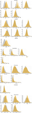
TABLE 2. Average R2, root mean square error (RMSE), and mean absolute error (MAE) ± standard deviation for the age prediction models within the training sample (Cam-CAN), test set, and age-corrected test set Training sample (Cam-CAN) Test set before age-bias correction Test set after age-bias correction DTI R2 .82 ± .04 .72 .92 RMSE 7.67 ± 0.83 10.11 5.12 MAE 6.15 ± 0.55 8.37 4.06 T1 R2 .81 ± .04 .73 .87 RMSE RMSE 9.11 6.55 MAE MAE 7.2 5.21 3.2 Cardiometabolic risk factors 3.2.1 Descriptive statistics TABLE 3. Descriptive statistics at baseline for each variable bar smoking, which is summarized in its own table due to its ordinal nature Mean ± SD Min Max Hematology Hemoglobin 14.2 ± 1.2 9.8 18.6 MCHC 33.2 ± 1 29 36 MCV 90.6 ± 3.9 76 108 MCH 30 ± 1.4 22.2 36.7 Thrombocytes 255.8 ± 55.4 81 499 Electrolytes Phosphate 1.1 ± 0.2 0.5 1.6 Calcium 2.4 ± 0.1 2.1 2.9 Sodium 140.6 ± 2.1 131 147 Chloride 101.6 ± 2.2 93 107 Magnesium 0.9 ± 0.1 0.6 1.1 Potassium 4.3 ± 0.3 2.9 5.9 Metabolites Creatinine 74.7 ± 13 46 115 Enzymes/Markers ALAT 24.7 ± 12.3 3 97 CK 126.7 ± 75 31 499 LD 168 ± 29 83 293 GT 24.7 ± 17.4 5 149 Carbohydrates Glucose 5.3 ± 0.8 2.3 10.6 Proteins/Lipids HDL cholesterol 1.6 ± 0.5 0.6 4.4 Total cholesterol 5.1 ± 1.1 2.9 8.9 LDL cholesterol 3.2 ± 0.9 1.2 6.4 CRP 1.6 ± 1.7 0.4 12.2 Triglycerides 1.3 ± 0.9 0.3 7.7 Clinical measures WHR 0.9 ± 0.1 0.5 1.3 Systolic 127.6 ± 17.5 90 190 Diastolic 80 ± 9.6 50 113.7 Pulse 66 ± 9.5 40 97.6 BMI 25.2 ± 4.1 16.8 43.4 TABLE 4. Smoking at baseline Frequency (%) Never smoked 593 (75.1) Previous smoker 127 (16.0) Current smoker 70 (8.9) Distribution of the cardiometabolic risk factors. Density plots for each variable, split by sex (male = orange, female = grey). Vertical lines represent mean values for each sex. See Table S3 for reference (normal/healthy) range for each variable
3.3 Bayesian multilevel models
3.3.1 Effects of time on brain age gaps
Distribution of the cardiometabolic risk factors. Density plots for each variable, split by sex (male = orange, female = grey). Vertical lines represent mean values for each sex. See Table S3 for reference (normal/healthy) range for each variable
3.3 Bayesian multilevel models
3.3.1 Effects of time on brain age gaps
Figure 4 shows predicted age for each model plotted as a function of age. Bayesian modeling revealed higher DTI (β = 0.24), and T1 (β = 0.19), based BAG at follow-up than baseline (Figure S12).
留言 (0)