
記住我

Parkinson's disease (PD) is the second most common neurodegenerative disease in aging populations (Hayes, 2019). In its most classical manifestation, PD is characterized by progressive motor impairment (Kalia & Lang, 2015), which results from abnormalities of the basal ganglia circuits due to the death of dopaminergic neurons in the pars compacta of the substantia nigra (Kalia, Brotchie, & Fox, 2013). However, pathophysiological changes outside of the basal ganglia are widely acknowledged to also have significant roles in modulating motor loops (Bartels & Leenders, 2009; Guan et al., 2019; Kalia et al., 2013). Moreover, complex within-network segregation and between-network coupling might significantly contribute to motor disorder, but in such a large-scale brain network view, the potential network underpinning for PD is not well investigated, and little is known about the intricate interactions between or within distinct networks.
Resting-state functional magnetic resonance imaging (rs-fMRI) has provided an approach to studying the central processing of motor impairment in vivo. In numerous studies, rs-fMRI has been used to identify associations between motor impairment and functional connections in classical motor regions such as the basal ganglia and motor cortex (Hacker, Perlmutter, Criswell, Ances, & Snyder, 2012; Nachev, Kennard, & Husain, 2008), as well as in non-motor regions including the frontoparietal and visual networks and the limbic system (Gilat et al., 2018; Kann, Chang, Manza, & Leung, 2020; Tessitore et al., 2012; Vervoort et al., 2016). However, the findings vary greatly. One of the main concerns is that PD patients recruited into these studies have already been exposed to dopaminergic medication, which would lead to heterogeneous reorganizations of brain function in order to preserve motor behavior (Krismer & Seppi, 2021; Tahmasian et al., 2015). This important influence has been widely ignored. Therefore, we hypothesized that studies in drug-naïve patients are a priority for investigating the intrinsic and complex interactions between/within district networks that relate to motor impairment, and might provide a robust prediction of motor impairment when the influence of medication is subsequently taken into consideration.
Moreover, because the neurodegenerative process acting on the human brain has little consensus between individuals, progresses along different trajectories, and is complicated by various pathophysiological factors, more attention has been paid to personal brain organization. Finding a link between an individual functional connectome and behavioral measurements can maximally reduce the bias inherent in population variation, and the resulting brain–behavior associations observed would be more robust and generalized (Tessitore, Cirillo, & De Micco, 2019). Thus, a connectome-based predictive modeling (CPM) approach has been newly introduced to predict behavior at the individual level by using large-scale network functional connectivity in a machine-learning framework. This has been used to investigate the complex mechanisms underlying mental and cognitive disorders (Gao et al., 2020; Ren et al., 2021; Yu et al., 2020), as well as in predicting outcomes after deep brain stimulation in PD patients (Shang, He, Ma, Ma, & Li, 2020). Therefore, by taking advantage of a CPM framework built on informative large-scale network connections, a novel predictive model would be constructed for identifying intrinsic network patterns for drug-naïve patients, which might have robust performance in predicting motor impairment.
Hence, this study aimed to construct a whole-brain connectome model that can predict motor impairment in PD patients. In order to reveal the disease-intrinsic functional underpinnings free of the effects of dopaminergic medication, we constructed a predictive model on drug-naïve patients and tested its performance in an independent group of drug-managed PD patients to check its reliability.
2 METHODS 2.1 Participant enrollment and evaluationAll patients signed informed consent forms in accordance with the approval of the Medical Ethics Committee of the Second Affiliated Hospital of Zhejiang University School of Medicine.
Two hundred PD patients were initially recruited to this study. The diagnosis of PD was made by a senior neurologist (B. R. Z.) according to the United Kingdom Parkinson's Disease Society Brain Bank criteria (Hughes, Daniel, Kilford, & Lees, 1992). Twenty-four patients were excluded on the basis of having either (a) cerebrovascular disorders, including previous stroke, history of head injury, or other neurological diseases (N = 14); or (b) cognitive impairment based on the Mini-Mental State Examination (MMSE), estimated by the criteria applicable to the Chinese population (MMSE score ≤ 17 for illiterate patients, ≤20 for grade-school literates, and ≤23 for junior high school and higher education literates [N = 10]) (Katzman et al., 1988; M. Y. Zhang et al., 1990). A final total of 176 PD patients were enrolled in this study, comprising 49 drug-naïve and 127 drug-managed patients. Drug-managed PD patients underwent clinical assessment on the morning after all dopamine replacement therapy was withdrawn overnight (at least 12 hr into their “drug-off status”). Basic demographic information, including age, gender, level of education, and duration of disease, and neurological and psychiatric scales including Unified Parkinson's Disease Rating Scale Part III (UPDRS III) score, Hoehn and Yahr stage (H–Y stage), and MMSE score were obtained for all patients. The total levodopa equivalent daily dose (LEDD) (Tomlinson et al., 2010) and duration of treatment were recorded for drug-managed patients.
2.2 Image acquisition and preprocessing 2.2.1 Image acquisitionAll imaging data were acquired on a 3.0 T magnetic resonance imaging (MRI) scanner (Discovery MR750, GE Healthcare). MRI scanning of each drug-managed patient was carried out in the drug-off status. The head of each participant was stabilized with foam pads, and earplugs were provided to reduce audible noise during scanning.
rs-fMRI data were acquired using gradient recalled echo–echo planar imaging sequence: echo time = 30 ms; repetition time = 2,000 ms; flip angle = 77°; field of view = 240 × 240 mm2; matrix = 64 × 64; slice thickness = 4 mm; slice gap = 0 mm; number of slices = 38 (axial); time points = 205. Structural T1-weighted images were acquired using a fast-spoiled gradient-recalled sequence: echo time = 3.036 ms; repetition time = 7.336 ms; inversion time = 450 ms; flip angle = 11°; field of view = 260 × 260 mm2; matrix = 256 × 256; slice thickness = 1.2 mm; number of slices = 196 (sagittal). All the sequence fields of view covered the whole brain, including the cerebrum, cerebellum, and brain stem.
2.2.2 Image preprocessingRs-fMRI data processing was carried out using Statistical Parametric Mapping (SPM 12, https://www.fil.ion.ucl.ac.uk/spm/) and Data Processing Assistant for Resting State fMRI (DPABI_V3.1_180801, http://www.rfmri.org/) (Yan, Wang, Zuo, & Zang, 2016). In an initial step, the first 10 volumes of the functional time series were deleted to utilize the MRI signal at equilibrium. The remaining images underwent slice timing for interval scanning, realignment, and normalization to the standard MNI space through T1 image segmentation. Next, spatial smoothing with a Gaussian kernel of 6 × 6 × 6 mm full width at half-maximum, detrending, covariate regression (Friston 24-motion parameters, mean signals of white matter and cerebrospinal fluid), and band-pass temporal filtering (0.01–0.1 Hz) were sequentially applied to the remaining volumes.
2.2.3 Control of head motionTo account for the effect of head motion on the rs-fMRI analysis, volumes with mean frame-wise displacement (FD) ≥ 0.2 mm were removed, and the remaining volumes were used for network construction. Then, 14 individuals—2 drug-naïve and 12 drug-managed patients—having <4 min (120 volumes) of data after scrubbing were excluded from the following analysis (Jenkinson, Bannister, Brady, & Smith, 2002; Parkes, Fulcher, Yücel, & Fornito, 2018). Consequently, a total of 162 PD patients were enrolled in this study, comprising 47 drug-naïve and 115 drug-managed patients. To verify that neither the observed nor the predicted scores were correlated with head-motion, correlation coefficients were calculated between the mean FD and observed and predicted scores, respectively. To further control for possible head-motion effects, we also applied a prediction analysis with the mean FD as an additional nuisance variable within the candidate connection selection process described in Section 2.3.1.
2.2.4 Functional network constructionConsistent with previous CPM-based studies, network nodes were defined using the 268-region-of-interest functional brain atlas (Shen, Tokoglu, Papademetris, & Constable, 2013). This atlas covers the whole brain, including cortical, subcortical, and brainstem structures. The whole-brain functional connection matrix was constructed for each patient in the MNI space. The mean time series of each node was extracted by averaging the time series of all voxels in each defined node. The functional connection was then calculated as the Pearson correlation coefficient (r) between the mean time series of each pair of nodes. Both positive and negative correlation coefficients were included to construct the connection matrix. A Fisher's r-to-z transformation was then used to normalize the correlation coefficients, and the resulting 268 × 268 matrix for each participant was utilized for the subsequent CPM analysis. Each element of the matrix represented the strength of connection between two nodes.
2.3 Connectome-based model construction and evaluation in drug-naïve patientsA flowchart for the construction of the connectome-based model and its evaluation is shown in Figure 1. All processes were performed by applying free scripts in MATLAB (R2020b for Windows, MathWorks). These scripts are available at https://www.nitrc.org/projects/bioimagesuite/.

Workflow for identifying a whole-brain connectome-based model for predicting motor impairment in PD. Model M was first constructed and evaluated among drug-naïve PD patients. Its predictive performance was further validated among drug-managed PD patients for reliability checking. LOOCV, leave-one-out cross-validation; PD, Parkinson's disease; UPDRS III, the Unified Parkinson's Disease Rating Scale Part III
2.3.1 Selection of candidate connections by using a leave-one-out cross-validation procedureAcknowledging the relatively small number of drug-naïve patients (N = 47), a leave-one-out cross-validation (LOOCV) procedure was used to select candidate connections (Rosenberg et al., 2016; Scheinost et al., 2019). The LOOCV procedure was repeated iteratively. In each iteration, one patient was removed from the training set and data for the remaining N − 1 patients were used for testing according to the following steps. First, the correlation between the strength of each connection and the observed UPDRS III score was assessed. In this step, Spearman's analysis was applied since the observed scores in this study were not normally distributed (Kolmogorov–Smirnov test, p < .05) (Shen et al., 2017). A partial correlation analysis was also conducted to ensure that the constructed model captured meaningful connection alternation associated with motor impairment (Scheinost et al., 2019). Three nuisance variables correlating with the phenotypic measure or neuroimaging data were included: age (significantly correlated with UPDRS III scores), duration (significantly correlated with UPDRS III scores), and gender (shown by Zhang, Dougherty, Baum, White, and Michael (2018) to affect functional connections). Next, the connections were selected based on the significance of the correlation between the connection strength and UPDRS III score. The significance threshold of p value was optimized to afford the best predictive performance (detailed in Section 2.3.4). Finally, all selected connections were categorized as either positive connections (connections for which strength indexed with higher UPDRS III score and severe motor impairment) or negative connections (the strength of which indexed with lower UPDRS III score and milder motor impairment) according to their correlation coefficients with observed scores. The above-mentioned steps were repeated N times (N = 47) until all patients had been excluded.
2.3.2 Model construction with consensus connections and prediction evaluation After the LOOCV procedure was performed, 47 sets of candidate connections were obtained. Owing to the nature of cross-validation, a slightly different set of candidate connections can be selected in different iterations. To reduce potential variation, the connections finally utilized for model construction should be selected in each iteration, and are termed “consensus connections.” These connections had the highest reliability among all candidate connections. All positive consensus connections and negative consensus connections were marked to construct respective binary masks. These two masks were then applied to each patient's own matrix to calculate the sum strengths of the positive and negative consensus connections. Summed strengths of positive and negative consensus connections were then fit with general linear regression to build a relationship with the observed score. The predicted score of each patient could be calculated by applying the constructed linear model with the following formula: where
where  is the sum of the strengths of positive consensus connections and
  is the sum of the strengths of negative consensus connections.
The performance of the constructed model was evaluated by calculating the Spearman correlation coefficient (rtrue) and the mean squared error (MSE) between observed and predicted UPDRS III scores. The values of a correlation coefficient and the MSE are usually dependent, that is, a higher correlation implies lower MSE and vice versa. A lower MSE value means that the difference between the predicted and observed scores is smaller (Shen et al., 2017). The significance of the constructed model was further tested by applying the 1,000-permutation test (Ren et al., 2021), which involved randomly shuffling the UPDRS III score and repeating the above processes 1,000 times. The significance of the permutation test was analyzed by calculating the percentage of sampled permutations that were greater or equal to the rtrue value (ppermu); ppermu < .05 was considered statistically significant.
2.3.3 Prediction comparison among connectome-based models constructed using different methodsWe sought to determine (a) whether a model constructed with a combination of positive and negative connections performs better than a model constructed with only positive or negative connections, and (b) whether models constructed with consensus connections selected in all iterations (representing highest reliability) perform better than models constructed with candidate connections in each iteration (representing less reliability). To these ends, the predictive power of model M was compared with other three models: model M1 constructed with positive consensus connections, model M2 constructed with negative consensus connections, and model M3 in which predicted scores were generated from each LOOCV iteration. Optimization of the threshold and permutation testing were also applied during the construction of M1, M2, and M3. Thus, the thresholds of these four models can vary. The processes for constructing models M1, M2, and M3 are detailed in the supporting information. To determine whether the predictive power of these models was significantly different from model M, Steiger's Z test was used to compare the rtrue value of model M with those of the other three (Rosenberg et al., 2016).
2.3.4 Optimal threshold valueFor selection of candidate connections, rather than applying an arbitrary p value threshold as did a previous study (Rosenberg et al., 2016), predictive ability was compared using different p value cutoffs. These thresholds were evaluated by repeating the above process 50 times using p values ranging from .05 to .001, with intervals of .001. The p value that afforded the highest rtrue value (the correlation coefficient between predicted and observed UPDRS III scores) was selected and used in construction of the model.
2.4 Model validation in drug-managed patientsFinally, the model with the best predictive ability among the above-mentioned four was further validated in drug-managed patients. Correlation coefficient r and the MSE between observed and predicted scores were also calculated. The significance of r was calculated using standard parametric conversion, and p < .05 was considered statistically significant.
2.5 Functional network anatomy of the constructed connectome model 2.5.1 Grouping nodes into seven functional networksThe 268 nodes were divided into seven canonical functional networks according to anatomical order and previous studies (Lake et al., 2019; Shen et al., 2013), which were: frontoparietal (63 nodes), default mode (20 nodes), motor (50 nodes), visual-related (45 nodes), limbic (30 nodes), basal ganglia (29 nodes), and cerebellum (31 nodes) networks. The visual-related network comprised visual I, visual II, and visual association networks. A map of these seven networks is shown in the supporting information (Figure S1). Connections within each network (“within-network connections”) were calculated by summarizing the number of connections between nodes of that same network. Connections between two distinct networks (“between-network connections”) were calculated by summarizing the number of connections between nodes from different networks.
2.5.2 Contribution of each functional networkWe weighted each functional network's contribution by calculating the sum of positive consensus and negative consensus connections belonging to it; a greater number of connections indicate a greater contribution. To further assess the importance of each functional network to the prediction of motor impairment, we computationally “lesioned” the model to exclude connections from it. Accordingly, in an iterative analysis, we masked the connection matrix to exclude connections that appeared in one of the seven functional networks. For example, after excluding connections in the frontoparietal networks, which contained 63 nodes, a 205 × 205 matrix rather than a 268 × 268 matrix was submitted for analysis. Models with lesioned matrices, termed “lesioned models,” were first constructed and evaluated among drug-naïve patients and then validated with drug-managed patients. The predictive ability of each lesioned model was evaluated according to the correlation between the predicted and observed UPDRS III scores, and the significance of the prediction was confirmed by permutation test in drug-naïve patients. The predictive ability of the lesioned model was compared with the original model by using Steiger's test. All p values were adjusted using a 14-comparison Bonferroni correction.
2.5.3 Two connection patterns from the connectome modelTo better understand the relationships between motor impairment in PD and various within- and between-functional connections, we divided the connectome model into two connection patterns. One pattern that contained all the negative consensus connections was called the “negative motor-impairment-related network.” The other pattern, containing all the positive consensus connections, was called the “positive motor-impairment-related network.” The characteristics of within- and between-network connections were analyzed by summing the consensus connections using the above-mentioned seven canonical functional networks in the positive and negative motor-impairment-related networks. To control the effect of variation in network size, the proportion of the connections within and between networks was also calculated by dividing the actual number of connections by the total number of possible connections (Gao et al., 2020).
2.6 Statistical analysesThe clinical characteristics of drug-naïve and drug-managed patients were analyzed by using SPSS software (version 25). A Kolmogorov–Smirnov test was applied to identify the normal distribution of continuous variables. Differences in normally distributed variables between the two groups were evaluated with the two-sample t test; otherwise, the Mann–Whitney test was conducted. Differences for qualitative variables were compared using the chi-square test. Statistical analyses of model construction, validation, and evaluation were performed in MATLAB (R2020b, MathWorks); details are given in the respective sections above. Unless stated otherwise, a two-sided p value <.05 was considered significant.
3 RESULTS 3.1 Characteristics of enrolled patientsA total of 162 PD patients were enrolled in this study, including 47 drug-naïve and 115 drug-managed patients. The characteristics of the patients in these two groups are summarized in Table 1. With the exception of treatment status (LEDD and duration of treatment), drug-managed patients had a significantly longer duration of disease (p = .005), higher H–Y stage (p < .001), and higher UPDRS III score (p = .002) compared with drug-naïve patients. No significant differences in age, gender, MMSE score, and level of education were observed between the two groups. Spearman correlation analysis demonstrated that UPDRS III scores of drug-naïve patients were significantly associated with age (r = .404, p = .004) and disease duration (r = .527, p < .001), which had been controlled by partial analysis in the process of candidate connection selection.
TABLE 1. Patients' characteristics Patient characteristic Drug-naïve group (N = 47) Drug-managed group (N = 115) p-Value Gender (male:female) 22:25 65:50 .061 Age (years, mean ± SD) 57.72 ± 10.085 60.44 ± 9.581 .109 Duration of disease (years, median (range)) 1.82 (0.08–10.25) 3.47 (0.08–26.37) .005* UPDRS III score (median (range)) 18 (4–68) 19 (3–66) .002* H–Y stage (median (range)) 2 (1–3) 2.5 (1–5) <.001* LEED (median (range)) — 425 (25–1,300) NA Duration of treatment (years, median (range)) — 2.04 (0.04–26.37) NA MMSE (median (range)) 28 (19–30) 28 (17–30) .497 Education (median (range)) 9 (0–18) 9 (0–18) .459 Note: p < .05 was considered statistically significant (annotated with *). Abbreviations: H–Y stage, Hoehn and Yahr stage; LEDD, levodopa equivalent daily dose; MMSE, Mini-Mental State Examination; NA, not available; UPDRS III, the Unified Parkinson's Disease Rating Scale Part III. 3.2 Constructing and evaluating models in drug-naïve patients 3.2.1 Optimal threshold for selecting connectionsThe optimal threshold for maximizing the rtrue values of models M, M1, M2, and M3 was identified after repeating the model construction process with connection-selection thresholds of p values ranging from .05 to .001. In addition, the MSE value under each threshold within these four models was calculated to further evaluate the predictive accuracy. The optimal p value thresholds of M, M1, M2, and M3 were .009, .008, .001, and .001, respectively. In general, there appeared to be a consistent inverse relationship between rtrue and the MSE, which meant that the p value associated with the highest rtrue value was highly similar to that associated with a low MSE value. The rtrue and MSE values across the tested range of p values are shown in Figure S2.
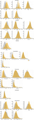
3.2.2 Prediction evaluation and model comparisonThere were 115 consensus connections selected to construct model M, including 58 negative consensus connections and 57 positive consensus connections (Figure 2). The strengths of positive and negative consensus connections significantly correlated with UPDRS III scores (positive connections: r = .712, p < .001; negative connections: r = −.661, p < .001; Figure S3). The highest sum of selected connections was obtained for model M, representing 0.32% of the sum (35,778) of whole-brain connections. The significant correlation between the observed and predicted UPDRS III scores demonstrated that the constructed model could predict the severity of motor impairment in individual drug-naïve PD patients (rtrue = .845, p < .001, ppermu = .002, MSE = 137.57; Figure 3, drug-naïve group). After controlling for clinical characteristics (including age, gender, disease duration, H–Y stage) within a partial correlation analysis, the predicted scores remained significantly associated with the observed scores (r = .763, p < .001).
 The constructed model M contained 57 positive consensus connections (pink) and 58 negative consensus connections (blue). Connectivity figures were created using the tool available at http://bisweb.yale.edu/connviewer/

The constructed model M could predict individual motor impairment severity of drug-naïve and drug-managed patients. Both predicted and observed scores were standardized for visualization. UPDRS III, the Unified Parkinson's Disease Rating Scale Part III
Compared with models M1, M2, and M3, model M had a significantly higher rtrue value (Table 2 and Figure S4). Furthermore, model M contained all consensus connections selected by M1 and M2. These results suggest that model M contained reliable and valuable information reflecting the core functional underpinnings associated with motor impairment, which afford the best predictive performance in the drug-naïve group.
TABLE 2. Comparison of predictions from connectome-based models Model rtrue (p, ppermu) MSE Steiger's Z value p-Value M .845 (<.001, .002) 137.57 — — M1 .712 (<.001, .014) 182.83 2.63 .008* M2 .711 (<.001, .012) 159.95 2.39 .017* M3 .528 (<.001, .002) 248.69 4.44 <.001* Note: rtrue is the true predictive correlation coefficient between observed and predict scores; ppermu is the p value obtained from permutation test (1,000 times); *p < .05 was considered statistically significant. Abbreviation: MSE, mean squared error. 3.2.3 Head motion controlThe head motion of each patient, which was evaluated by calculating mean FD, was not significantly associated with either observed scores (r = .031, p = .837) or the predicted scores generated with model M (r = .045, p = .762). Furthermore, in combining the mean FD as an additional nuisance variable when selecting candidate connections, the constructed model remained predictive for drug-naïve patients (rtrue = .835, p < .001, ppermu = .001, MSE = 135.73). The predictive performance of this model was not significantly different from the original (Steiger's Z value = 1.936, p = .053). In addition, the common connections were highly overlapped with the network of model M after controlling for head motion (percentage overlap: higher-UPDRS III score network 94.7%, lower-UPDRS III score 91.4%). These results suggest that head motion did not have significant confounding effects on our principal results.
3.3 Validating the constructed model in drug-managed patientsModel M significantly predicted UPDRS III score in the independent drug-managed group (r = .209, p = .025, MSE = 182.96; Figure 3). This result remained stable after introducing head motion as a nuisance variable in the candidate connection selection process (r = .219, p = .019, MSE = 182.17) and did not significantly differ from the original (Steiger's Z value = 0.626, p = .535). These results demonstrated that head motion did not significantly affect the predictions of model M in drug-managed patients. Furthermore, after controlling clinical characteristics (including age, gender, disease duration, H–Y stage, LEDD, and duration of treatment) within partial correlation analysis, the predicted scores generated with model M remained significantly associated with the observed scores (r = .214, p = .025).
3.4 A hybrid model combining clinical factors with the constructed model MThe value of using the clinical factors age, gender, disease duration, and H–Y stage for prediction were evaluated by adding them into model M. By combining the sum of positive consensus connections and the sum of negative consensus connections with these four clinical factors, the hybrid model successfully predicted UPDRS III score in both drug-naïve (rtrue = .961, p < .001, ppermu < .001) and drug-managed groups (rtrue = .459, p < .001). The significant improvement of predictions detected in both groups demonstrated the value added by including clinical factors (drug-naïve group: 0.845 vs. 0.961, p < .001, drug-managed: 0.209 vs. 0.459, p < .001).
3.5 Analysis of functional network anatomy 3.5.1 Contribution of each functional network to prediction of motor impairmentBy summing positive and negative consensus connections together, we found that the motor network contributed predominantly, followed by the frontoparietal and limbic networks. After controlling for network size, the results consistently showed that the motor, limbic, the frontoparietal networks were the top three contributors to the connectome model (Figure S5). Next, we tested the importance of each individual functional network for predicting motor impairment by constructing lesioned models (Table 3). Compared with the whole-brain connectome model, in the drug-naïve group, the predictive power of the lesioned model was reduced after excluding visual-related (Steiger's Z value = 2.246, p = .025) and frontoparietal (Steiger's Z value = 2.149, p = .032) networks. In the drug-managed group, the predictive power was reduced after excluding the basal ganglia network (Steiger's Z value = 2.232, p = .026). The results of the Steiger's test did not remain significant after Bonferroni correction. These results demonstrate that the constructed model did not rely on the strength of a single functional network, but rather it incorporates information related to motor impairment from various neural networks throughout the brain.
TABLE 3. Predictions from lesioned models constructed from drug-naïve patients and validated on drug-managed patients Drug-naïve group Drug-managed group r, ppermu Z, p r, p Z, p Whole brain .845, .002 — .209, .025 — Lesioned model −FP .811, .001 2.149, .032 .202, .031 0.205, .837 −DM .845, .001 0, 1.0 .202, .030 0.535, .592 −Mot .809, .002 1.426, .154 .147, .117 1.110, .267 −Vis .819, .003 2.246, .025 .209, .024 0.961, .049 −Lim .836, .001 0.587, .557 .195, .036 0.639, .523 −BG .845, .001 0, 1.0 .192, .039 2.232, .026 −Cer .843, .001 0.695, .392 .203, .029 0.838, .402 Note: Predictability of models constructed from drug-naïve patients were generated with consensus connections and remained significant by using the optimal threshold of model M (p = .009). Predictability was assessed by calculating Spearman correlation coefficients (r) between observed and predicted scores. The significance of the prediction was confirmed by permutation testing in drug-naïve patients (ppermu). Predictability from whole-brain matrix is included in the first row for comparison. Results of Steiger's tests did not remain significant after Bonferroni correction. Abbreviations: BG, basal ganglia network; Cer, cerebellum network; DMN, default mode network; FP, frontoparietal network; Lim, limbic network; Mot, motor network; Vis, visual-related network. 3.5.2 Investigating connection patterns of the constructed modelWe then examined the connection patterns within and between the seven functional networks in the positive and negative motor-impairment-related networks by taking network size into consideration and obtaining the proportion of connections that each network contributes (Figure 4).

Negative (left, blue) and positive motor-impairment-related networks (right, pink). To control for the possible effects of network size, the proportions of the within- and between-network connections were obtained by dividing the actual number of connections by the total number of all possible connections. Each solid circle represents a functional network; thicker circles and lines represent a greater proportion of connectivity. BG, basal ganglia network; Cer, cerebellum network; DMN, default mode network; FP, frontoparietal network; Lim, limbic network; Mot, motor network; Vis, visual-related network
Results showed that, in the negative motor-impairment-related network, the motor, visual-related, and default mode networks were the top three contributors of within-network connections to this pattern. This reflected the more segregated pattern for this network, which contained more within-network connections (26.35‰) than between-network connections (20.57‰; Table S1). By contrast, in the positive motor-impairment-related networks, connections between motor-frontoparietal, motor-basal ganglia, and motor-limbic networks were the highest contributions. This indicates a more integrated pattern for the positive motor-impairment-related network, involvin
留言 (0)