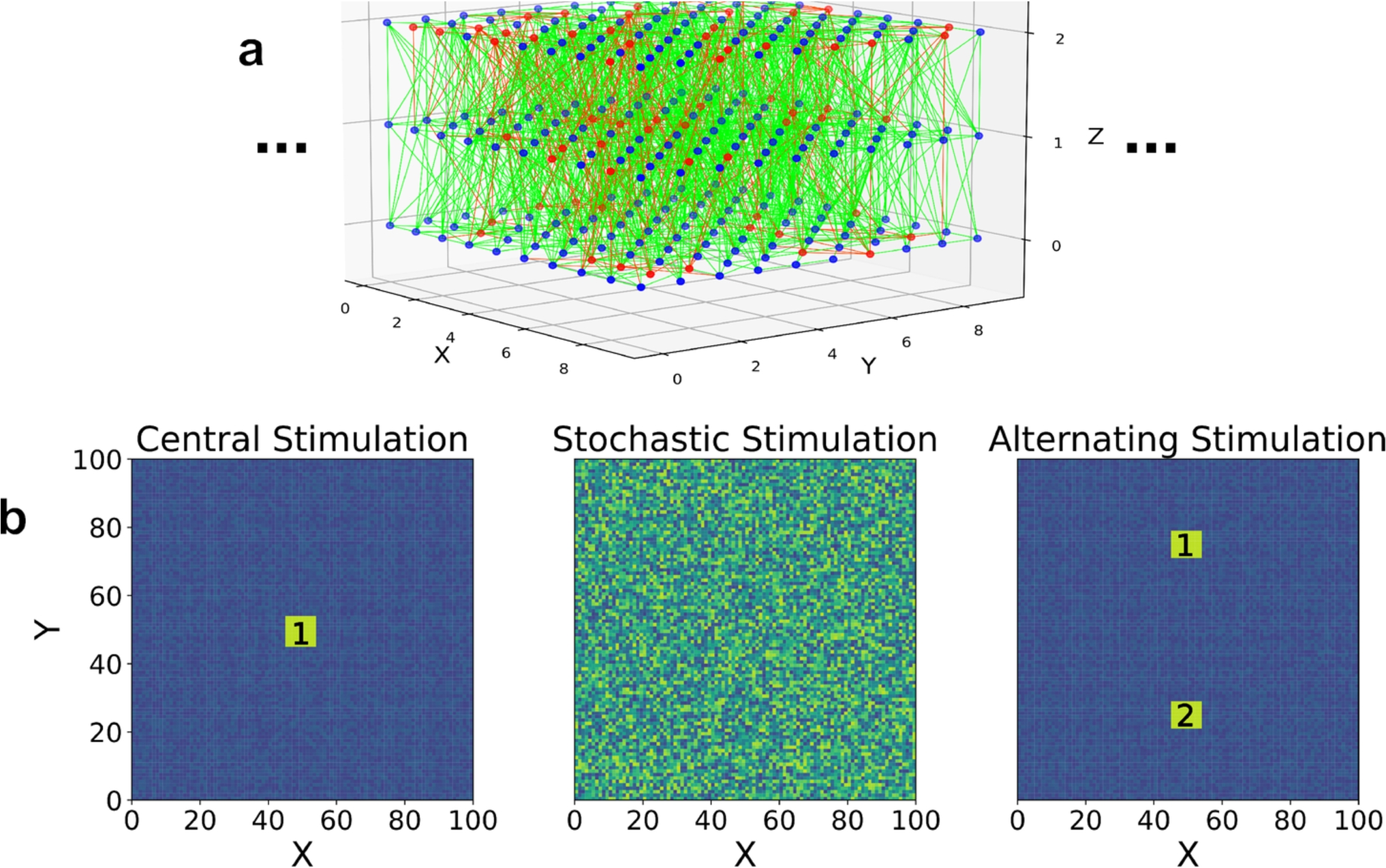
A schematic illustration of our model system is shown in Fig. 1A: The model network includes 200 inhibitory (blue) and 800 excitatory (red) neurons interconnected randomly with a sparsity of 0.1. The inhibitory neurons have a fixed value of weight (\(-1\)) for all efferent connections, while those of excitatory neurons dynamically vary from initially assigned value of 1.

Scatter plots of \(\sum }\) vs. \(\sum }\) depicting the evolution of the network morphology being subject to a \(S_0-S_1\) paired pulse (\(\Delta t^ = 3\) ms) conditioning. This sequence of snapshot plots illustrates the morphological transition depicted in Fig. 1D in the main text. The red and blue dots mark the subpopulation \(S_0\) and \(S_1\), respectively. The gray dots represent all other subpopulations. Note that during the given conditioning process, the network morphology fully stabilizes in about 600 seconds, after which only minor fluctuations occur

Our doublet conditioning procedure involves formulating 20 non-overlapping subpopulations \(S_i\) (i = 1, 2, ... , 20), each consisting of 50 neurons from the whole population of 1,000 neurons. A sequence of \(\) paired pulse electrical stimuli is then delivered to randomly chosen pairs of subpopulations \(S_i\) and \(S_j\) (\(i \ne j\)), with a time delay \( = 3\) ms; see the illustration in Fig. 1A. The interval between successive \(\) paired pulse stimuli (marked by black arrows on the top of each raster plot in Fig. 1B) is randomly chosen between 100 to 300 ms. In contrast, rewarded target \(\) paired pulse stimuli are administered (with an average interval of 76 s, marked by green arrows in Fig. 1B) only for a specific pair of subpopulations (e.g., \(S_0\) and \(S_1\)) with \(\Delta t = \Delta t^\) (= 3 ms); the subsequent dopamine reward is delivered with a significant time delay (randomly chosen) between 0 to 1000 ms (marked by magenta triangles in the lower horizontal axis of Fig. 1B) from the onset of each stimulus. This “distal reward” scheme works effectively because of the memory effect of the eligibility time trace \(C_\) (refer to Section 3).

It is also important to note that each random deterrent stimulation (indicated by black arrows in Fig. 1B) elicits spiking activity in numerous neurons, leading to synaptic weight modifications in the presence of residual dopamine, \(D_r\). However, the timing of these deterrent-induced spiking events is not aligned with (i.e., does not consistently repeat with) the dopamine reward timing. In contrast, the rewarded stimuli (green arrows in Fig. 1B) and the spikes they generate are temporally correlated with their respective distal rewards. A more detailed description of the model network and the Pavlovian conditioning process can be found in Section 3.

Figure 1B displays two raster plots illustrating population bursts in response to a series of paired-pulse \(\Delta t\) stimuli: the top row captures the early stage of conditioning, while the bottom row shows the fully conditioned late stage. Notably, after Pavlovian conditioning is complete, dopamine-rewarded paired-pulse stimulation (marked by the green arrow in the lower plot of Fig. 2B) produces a markedly enhanced population burst. This effect of conditioning is evident when comparing the two different green spike density function (SDF) lines in the second column of Fig. 1B; Fig. S1 in the supplementary materials, enlarged raster plots further detail the bursts marked by the two green arrows in Fig. 1B. The same SDF plots also display the average SDF profile of non-rewarded stimuli (black lines). During the early conditioning phase (top plot), the green and black SDF profiles overlap closely. However, after conditioning, the green SDF profile separates distinctly from the black SDF profile associated with non-rewarded doublet stimuli (bottom plot).

The strong inhibition about 100 ms duration (i.e., a system-wide refractory period with only a few spikes), immediately following the green arrow in the second row of Fig. 1B is a natural consequence of the network having just undergone a full-scale system-wide firing event (as shown by the large green SDF in the second column of Fig. 1B). As it will be carefully analyzed below, the fully conditioned network has acquired a strong feedforward structure, and the “green arrow stimulation” initiates coherent population firing activity from the top of the feedforward network that propagates all the way to its end. In contrast, non-rewarded (or non-conditioned) stimuli (represented by black arrows), delivered to non-targeted subpopulations that are more or less uniformly scattered across the entire network, do not trigger a system-wide firing avalanche: Essentially, the scattered, small fire seeds from these stimuli, when applied over the established feedforward network (or even the initial random network), fail to generate a significant avalanche event.

As the network gets conditioned with the sequence of rewarded stimuli, its morphology undergoes significant transformation, with approximately 50% of the initial excitatory connections reaching a nearly saturated weight about the maximum value of 4, while around 36% become inactive, with weights near zero (see Fig. 1C). The degree of weight saturation can be changed by adjusting some parameters, particularly those governing the STDP rule. In this study, near-binary saturation is advantageous as it simplifies the network’s graph analysis.

Of particular interest, the total excitatory weights of efferent connections (\(\sum }\)) and afferent connections (\(\sum }\)) for excitatory neurons display a strong negative correlation, as shown by the violet points in Fig. 1D. This represents a marked departure from the initial state, where the distribution is tightly clustered with \(\sum } \simeq \sum } \simeq \) 80, corresponding to a random network with 800 excitatory neurons at a connection sparsity level of 0.1. It is important to note that here both \(\sum }\) and \(\sum }\) reflect only excitatory connection weights; inhibitory connection weights, fixed at a value of -1 in this study, are excluded.

Encoding the value of \(\Delta t^\) into the network morphology. Neurons within \(S_0\) are colored in red, while those in \(S_1\) are colored in blue. It is noteworthy that the centers of \(S_1\) (blue dots) are systematically positioned along the negative slope of scattered dots, arranged sequentially based on their corresponding values of \(\Delta t^\) (see the last frame in the second row). For all values of \(\Delta t^\) within the range of \(0 \sim 10\) ms, the network exhibits a remarkably similar feedforward structure (that is, scatter plot with a strong negative correlation)

A fully conditioned steady state is typically reached within approximately 600 seconds, with some intermediate network states depicted in Fig. 2. Again, as the weight values approach saturation at either 0 or 4 (see Fig. 1C, purple), the network reconfigures into a nearly binary structure. Consequently, \(\sum }\) (\(\sum }\)) becomes linearly proportional to the respective outdegree (indegree) of each neuron, a feature that significantly simplifies the characterization of network morphology. In essence, in the fully conditioned network, the indegree of an excitatory neuron is anti-correlated with its outdegree.

The robust negative cross-correlation evident in the scatter plot of Fig. 1D (purple dots) provides compelling evidence that the fully conditioned network exhibits a pronounced feedforward (“synfire chain”) morphology, despite the coexistence of some recurrent connections, which confer the significant level of scatters in the direction perpendicular to the overall negative slope. The heuristic explanation is as follows. Naturally, the neurons of the subpopulation \(S_0\) (red dots), which receive the first stimulation pulse, are positioned at the apex of this feedforward hierarchy. Then, the neurons of \(S_1\) (blue dots), which receives the following second pulse, are being forced to position themselves about a downstream position which is set by the imposed time interval \(\Delta t (= 3)\) ms (again, see Fig. 2).

As the conditioning process progresses, the delivery of a rewarded \(S_0 - S_1\) paired pulse stimulation to the conditioned network consistently triggers a population burst with remarkable similarity. This similarity is characterized by more or less well-preserved relative temporal ordering of spiking events within the burst, while the exact spike timings change from one burst to others. The preserved firing order, coupled with the STDP potentiation (inhibition) mechanism, which acts specifically on causal (non-causal) events of pre- and post-synaptic firings, naturally facilitates the establishment of a feedforward network morphology (see the schematic illustration and its explanation in Fig. S2 of the supplementary materials for the establishment of the negative correlation among the purple dots in Fig. 1D). Another way to visualize the established feedforward network morphology is its weight matrix, which clearly reveals a wedge-shaped asymmetry associated with the established network [see Fig. S3 of the supplementary materials]. The pronounced feedforwardness is also vividly illustrated by the downward spread of the rewarded, paired pulse stimulation-induced population burst along the negative slope of \(\sum }\) vs. \(\sum }\) plot in Fig. 1E (Also, see the corresponding raster plot of Fig. S4 in the supplementary materials).

Given that we can condition the model network with a specific \(\Delta t^ = 3\) ms paired pulse stimulation applied to a set of two subpopulations (\(S_0\) and \(S_1\)) and that this conditioning process results in the formation of a feedforward network, we are prompted to investigate how the value of \(\Delta t^\) becomes encoded into the network. For that matter we have conditioned the model network for many different values of \(\Delta t^\). Figure 3, illustrating the positions of the two subpopulation groups (red: \(S_0\); blue: \(S_1\)) along the feedforward network for various values of \(\Delta t^\), provides a clear answer to the question. Despite noticeable scatter, points corresponding to the two distinct subpopulations exhibit a tendency to occupy specific regions on the plane of \(\sum }\) vs \(\sum }\). Notably, the centroid positions of the blue points (representing the \(S_1\) subpopulation) are systematically aligned along the negative slope of \(\sum }\) vs. \(\sum }\) in accordance with the corresponding values of \(\Delta t^\). Here we point out that the maximum value of \(\Delta t^\) is limited by the full width of the SDF of population burst, which is approximately 10 ms. It is noteworthy that the entire scatter plots remain consistent across different \(\Delta t^\) values, despite variations in the individual point locations. It’s also important to recognize that subpopulations (represented by gray dots in Fig. 3) other than \(S_0\) and \(S_1\) contribute to the overall alignment of the feedforward morphology. However, these non-targeted subpopulations are not confined to a specific localized area but are widely dispersed over the network. In a sense, they are driven to integrate into the network by the stimulus-triggered spiking actions of \(S_0\) and \(S_1\).

Once the network is conditioned with a specific value of \(\Delta t^\), we evaluated the “perceptual effects” of temporal perturbations by using \(\Delta t^\) values different from \(\Delta t^\) for paired pulse stimulation. Figure 4 illustrates this scenario for the case of \(\Delta t^ = 3\) ms conditioned network. All SDF profiles (solid black lines) in Fig. 4A exhibit a very small hump immediately following the \(S_0\) pulse stimulation (marked by a red vertical line) and a more prominent dominant hump, whose peak can occur either before or after the \(S_1\) pulse stimulation (marked by a blue vertical line). While these profiles are qualitatively similar, their distinctions are evident, as depicted by the corresponding \(\Delta \)SDF (= SDF\(^\) - SDF\(^\)) profiles (green lines). Here, we should point out that even for the unconditioned naïve network, different stimuli also generate different responses, but all are too small to be meaningful compared to those of the conditioned network (see Fig. S5 in the supplementary materials).

The nature of \(\Delta \)SDF can be characterized by two distinct measures. Firstly, the overall time shifts of the SDFs of the test cases with respect to that of \(\Delta t^ = 3\) ms are measured: for that matter the cross-correlation functions between SDF\(^\)s and SDF\(^\) are computed as shown in Fig. 4B; and the peak times \(\tau ^\)s corresponding to the maximum cross-correlation are measured. \(\tau ^\) steadily increases as a function of \(\Delta t^\) and reaches a saturation approximately at \(\Delta t^ = 8\) ms (see Fig. 4C). Secondly, we measure the overall shape changes in the SDFs (as shown in Fig. 5A). When the SDF\(^\) profiles (black lines) are time-shifted by their corresponding values of \(\tau ^\) and overlaid over the SDF\(^\) profile (gray) generated by the \(\Delta t^ = 3\) ms doublet stimulation, the shape changes incurred by the temporal detuning become clear. The solid red lines in Fig. 5A depict the error function \(\epsilon \) = (SDF\(_^\) - SDF\(^\))\(^2\), and its integrated value \(\epsilon ^\) is plotted as a function of \(\Delta t^\) in Fig. 5B.

Temporal shifts of SDF profiles subject to different \(\Delta t^\) stimuli. The network underwent Pavlovian conditioning with \(\Delta t^ = 3\) ms before each test. (A) The responses of the conditioned network to different \(\Delta t^\) stimuli are visualized through their corresponding SDF\(^\) profiles (solid black line). Below each SDF\(^\) profile, the \(\Delta \)SDF\(^\) = SDF\(^\) - SDF\(^\) is depicted in green (solid line), where SDF\(^\) represents the burst profile for the \(\Delta t^ = 3\) ms (highlighted with a shaded region). For all the lines shown in (A), the trial-by-trial variations are so minimal that the standard deviations over more than 20 trials are smaller than the thickness of the lines used in the plots. (B) The cross-correlation functions between SDF\(^\)s and SDF\(^\) are illustrated (inset: blown-up image of the highlighted box). (C) Overall, the SDF\(^\) profiles exhibit a leftward (rightward) shift with respect to the reference profile SDF\(^\) when \(\Delta t^\) < (>) \(\Delta t^ = 3\) ms. The maximum correlation time \(\tau ^\) appears to saturate around 8 ms

Shape changes of SDF profiles in response to different \(\Delta t^\) stimuli. The network underwent conditioning with \(\Delta t^ = 3\) ms before each test. (A) SDF\(^\) profiles (solid black line), obtained for various \(\Delta t^\) values, are time-shifted by the amount of their matching \(\tau ^\) and superimposed on the SDF\(^\) profile (solid gray line). The differences \(\epsilon \) = (SDF\(_^\) - SDF\(^\))\(^2\) are represented by solid red lines in (A), and their integrated values \(\epsilon ^\) are given in (B). The value of \(\epsilon ^\) appears to saturate around 8 ms

The perceptual effects of different temporal perturbations can also be compared in the spatiotemporal evolutions of the stimulation-evoked population bursts, as illustrated in Fig. 6. In the figure, the variable \(\sum }\) effectively serves as a space variable as the excitation propagates in the increasing direction of \(\sum }\), as well illustrated in Fig. 1E. In Fig. 6, the fraction of activated excitatory neurons in each bin (size of 25) of \(\sum }\) is plotted over time. The lines highlighted in green correspond to instances immediately (i.e., 1 ms after) following the delivery of \(S_1\) pulses. Evidently, different \(\Delta t^\) values used in paired pulse stimulation yield distinct spatiotemporal evolutions. To emphasize the differences, the \(\sum }\) locations of \(S_1\) are guided by a red circle at \(t = 4\) ms.

Distinct spiking activity evolutions in the \(\sum }\) space in response to various \(\Delta t^\) stimuli. Following complete conditioning with \(\Delta t^ = 3\) ms, diverse \(\Delta t^\) stimuli are administered, and the temporal evolution of the number fractions of excited neurons in each bin (size: 25) of \(\sum }\) is plotted. It is evident that their \(\sum }\)-temporal evolutions significantly differ for varying values of \(\Delta t^\). Notably, the red circled region emphasizes the discrepancy in the location of the S1 subpopulation along the \(\sum }\) axis

Up to this point, we have opted to utilize a case where \(^=3\) ms for the evaluation of perceptual distances associated with temporal perturbations (as illustrated in Figs. 4 and 5). However, experimentation reveals that altering \(^\) to other values, such as 5 (or 4) ms, does not fundamentally modify the overarching characteristics of temporal Pavlovian learning and subsequent temporal perturbations (refer to Figs. S6 and S7 in the supplementary materials). It is noteworthy that the meaningful dynamic range of \(^\) is naturally constrained by the SDF duration of the induced population burst, which approximates 10 ms in the current setting. Also, note that the given system requires a relatively long recovery time (around 200 ms) following each system-wide population burst.

The concept of Pavlovian conditioning for a single time interval doublet can be expanded to encompass more intricate temporal information. For instance, a triplet pulse stimulation, as depicted in the upper segment of Fig. 7, involves three distinct subpopulations – \(S_0\), \(S_1\), \(S_2\) – and two time intervals, \(^\) and \(^\). Previously for the doublet conditioning protocol we have used non-overlapping subpopulations \(S_i\), but for the case of triplet conditioning we allow a small degree of overlaps (refer to Section 3). As it will be shown, this much of overlapping does not hinder the conditioning process at all.

Figure 7 consolidates fully conditioned networks for various combinations of \(^\) and \(^\). Once again, an initially random network evolves into a noisy feedforward structure, where the temporally leading excitatory neurons of the \(S_0\) subpopulation occupy the top left-hand corner of the scatter plot. The overall feedforward network morphologies remain essentially consistent across different cases, with the positioning of neurons from \(S_0\) (red) to \(S_1\) (blue) and \(S_2\) (green) occurring sequentially along the negative slope of the scatter plots. Clearly, the locations of blue and green points systematically vary along the negative slope according to the matching values of \(^\) and \(^\) (see the overlaid frames in the last column of Fig. 7). In essence, the time information of \(^\) and \(^\) is effectively encoded onto the spatial configuration of the scatter plot.

Encoding the time information of triplet stimuli into the network morphology. Three different subpopulations (\(S_0, S_1, S_2\)) are stimulated in distinct sequential modes, each characterized by different values of \(^\) and \(^\). The crosses representing the centroid positions of the three subpopulations are marked in red for \(S_0\), blue for \(S_1\), and green for \(S_2\). The sizes of these crosses correspond to the standard deviations of the point scatters. Importantly, the centroid positions are systematically arranged in the scatter plots of \(\sum }\) vs \(\sum }\) based on their corresponding values of \(^\) and \(^\) (see the two frames in the last column)

In line with prior methodology, we undertake an assessment of the perceptual changes subject to different temporal perturbations, specifically the detuning of \(^\) and \(^\) values, on the induced SDF of the condition network. An extreme test case will be just delivering a single \(S_0\) pulse stimulation without its subsequent \(S_1\) and \(S_2\) pulse stimuli (thus, \(^\) and \(^\) are meaningless). Surely, we see a significant change in the SDF of the induced population burst (see Fig. S8 in the supplementary materials).

The top row of Fig. 8A presents a visualization of five distinct SDFs derived from distinct triplet pulse simulations, each employing a unique combination of \(^\) and \(^\). Importantly, these configurations differ from the reference case (shaded in cyan), where \(^\) and \(^\) coincide with \(^ = 3\) ms and \(^ = 3\) ms, respectively. In the lower portion of Fig. 8A, the \(\Delta \)SDFs (depicted by green lines) resulting from a total of 25 distinct triplet test stimuli are showcased. And Fig. 8B exhibits cross-correlation functions (left) and a map (right) illustrating the maximum correlation times \(\tau _\)s (between SDF\(^\)s and SDF\(^\)) for 36 different triplets of stimuli. Following a methodology akin to the analysis in Figs. 5 and 8C presents a map of \(\epsilon ^\), offering a quantitative measure of SDF shape changes in relation to the reference case. Three illustrative examples are provided above the map of \(\epsilon ^\) for a visual illustration. Notably, \(\tau _\) displays more heightened sensitivity to variations in \(^\) than to \(^\), while \(\epsilon ^\) experiences a more stiff change, approximately along the diagonal line \(^ = - ^ + 5\). The perceptual effects of different (\(^\), \(^\)) temporal perturbations are also evident in the spatiotemporal evolutions of the stimulation-evoked population bursts (refer to Fig. S9 in the supplementary materials).

Temporal shifts of SDF profiles under different stimulating sets of \(^\) and \(^\). The network underwent Pavlovian conditioning with \(^ = 3\) ms and \(^ = 3\) ms before each test. (A) Six exemplary SDF\(^\)s obtained by stimulating the conditioned network with different sets of (\(^\), \(^\)). Below each SDF\(^\) profile is \(\Delta \)SDF = SDF\(^\) - SDF\(^\) for 25 different sets of (\(^\), \(^\)). (B) Illustration of cross-correlation functions between SDF\(^\)s and SDF\(^\) (left) and the color map of maximum cross-correlation time \(\tau ^\). It is notable that \(\tau ^\) is more sensitive to \(^\) than \(^\). (C) Three exemplary SDF\(^\) profiles (solid blue line), obtained for three different sets of stimuli, are time-shifted by their matching \(\tau ^\) and superimposed on the SDF\(^\) profile (solid gray line). The color map of \(\epsilon \) = (SDF\(_^\) - SDF\(^\))\(^2\) is presented below

The dynamic range of \(^\) (or \(^\), \(^\)) for the current doublet (or triplet) conditioning, typically \(\sim 10\) ms (or \(3 \sim 5\) ms), can be substantially extended when the stimulation-induced response transitions from a single-peak population burst to a superburst characterized by multiple peaks in its SDF profile and a substantially longer SDF duration. A superburst dynamic state can be easily achieved by incorporating an axonal conduction delay (e.g., 5 ms) across all synaptic connections in the previously used Izhikevich network.

The modified network can also be successfully conditioned with the same \(S_0-S_1-S_2\) triplet stimulation protocol but with much longer time intervals. As an example a target \(S_0-S_1-S_2\) triplet stimulation-triggered superburst in a fully conditioned network (with \(^ = ^ = 11\) ms) is illustrated in the raster plot of Fig. 9A (top), where each color-red, blue, green, and gray-represents subpopulations \(S_0\), \(S_1\), \(S_2\), and all other neurons, respectively. The corresponding SDFs for each subpopulation, which clearly peak at different time points, are shown in Fig. 9A (bottom). The SDFs of the remaining subpopulations (gray) and that of the combined total population (black) are also illustrated in the same graph.

Similar to those depicted in Figs. 7 and 9B shows a scatter plot of \(\sum W_\) versus \(\sum W_\) illustrating the network’s overall feedforward structure, characterized by a strong negative correlation between \(\sum W_\) and \(\sum W_\). Then, in Fig. 9C distinctive SDF profiles are shown for four different cases: the colors, pink, cyan, and brown represent cases where \(S_0\), \(S_1\), or \(S_2\) are stimulated separately at \(t = 0\), while black corresponds to sequential stimulation of all three with \(^ = ^ = 11\) ms. Note that naturally the impact of stimulation \(S_0\) is far greater than that of stimulation \(S_1\) or \(S_2\) as the subpopulation \(S_0\) sits at the apex of the conditioned network (refer to the red dots in Fig. 8B).

Figure 9D and E illustrates the highly diverse superburst SDF profiles, each averaged over 20 trials during the test phase after a full conditioning with \(^ = ^ = 11\) ms. We consider two different sets of test. Figure 9D shows SDF profiles for different \(S_0-S_1-S_2\) triplet stimuli, each with unique combinations of \(^\) and \(^\) values, illustrating a wide shape variation. Similarly, Fig. 9E compares superburst SDF profiles for different \(S_i-S_j-S_k\) triplet stimuli with the same values of \(^ = ^ = 11\) ms but with different combinations of subpopulations. Notably, random combinations of subpopulations other than \(S_0-S_1-S_2\) produce a significantly reduced SDF amplitude.

\(S_0-S_1-S_2\) triplet conditioning for a superburst-generating Izhikevich network and increased dynamic range of time-interval. The Izhikevich network, incorporating axonal conduction delays, was fully conditioned using the \(S_0-S_1-S_2\) triplet protocol with \(^ = ^ = 11\) ms. All test results shown in this figure are obtained after the network was fully conditioned. (A) The top panel shows a sample raster plot of a superburst triggered by the \(S_0-S_1-S_2\) stimulus with \(^ = 11\) ms and \(^ = 11\) ms (color-coded as follows: red for \(S_0\), blue for \(S_1\), green for \(S_2\), and gray for all other subpopulations). The bottom panel displays SDF profiles for each subpopulation, with colors corresponding to those in the raster plot. (B) Scatter plot showing \(\sum W_\) versus \(\sum W_\) of the conditioned network. (C - E) SDF profiles generated by various test stimuli: (C): different subpopulation(s) as indicated; (D) varying \(^\) and \(^\); (E) triplet stimuli with different combinations of subpopulation as labeled

Finally, since the range of short input time intervals (\(0 \sim 40\) ms) targeted in this work overlaps with the typical range of neuron membrane time constants, we tested several values of capacitance (C), as the quadratic Izhikevich neuron model we employed does not explicitly include a time constant. We found that as long as C was within the range of \(0.8 \sim 1.5\) nF (default value: 1.0 nF), the conditioning mechanism yielded qualitatively consistent results. Similarly, we tested various values for the STDP time constants (\(\tau _+\) and \(\tau _-\)) and observed that, as long as they were within the range of \(10 \sim 30\) ms (default value: 20 ms), the phenomena remained essentially unchanged.