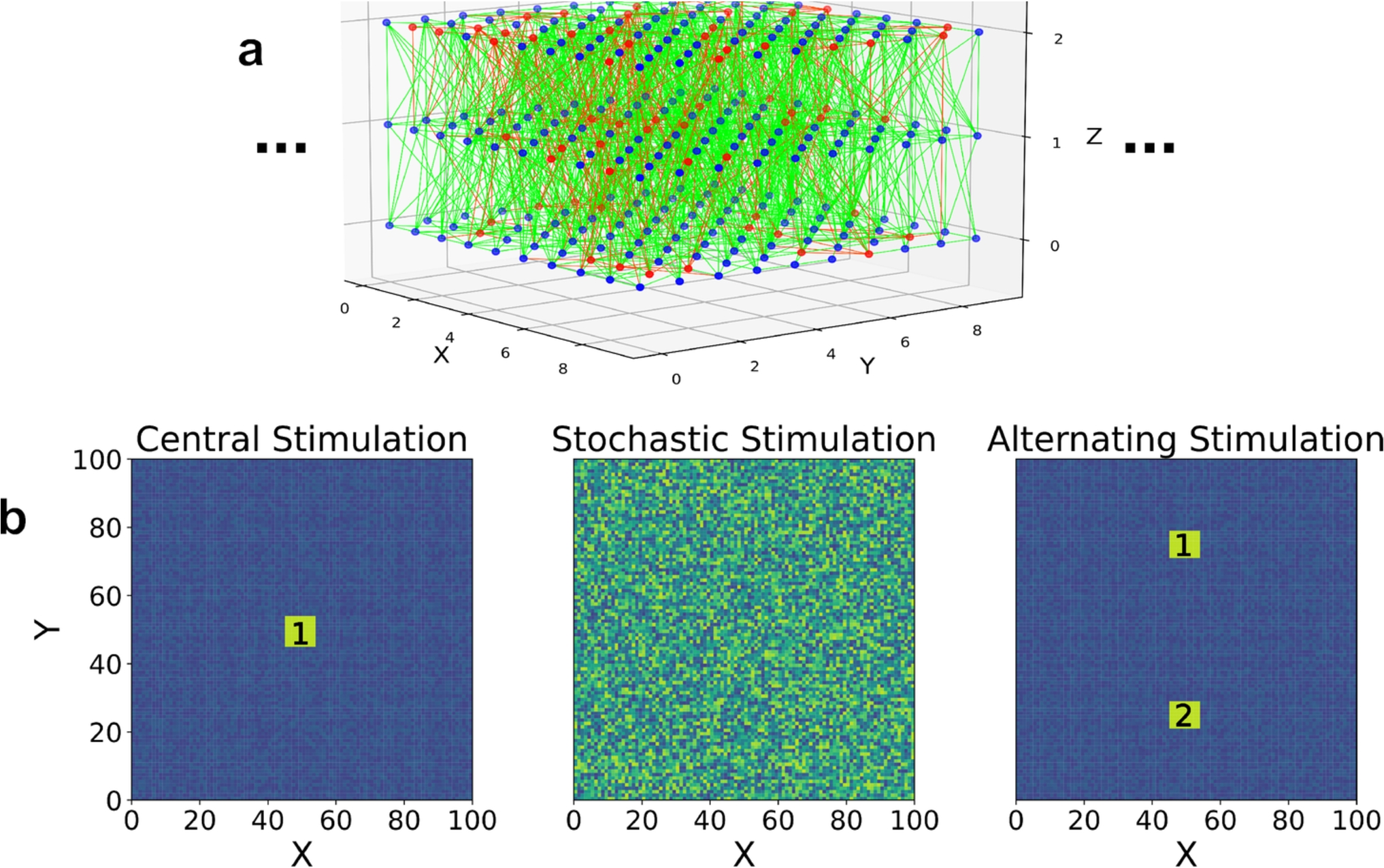
To study traveling waves in 2-dimensions, we construct a quasi-2D spiking network with random connections, local connection probability, and realistic spiking responses using the BRIAN neural simulator version 2.6.0 (Stimberg et al., 2019)Footnote 1 This network is constructed by placing model neurons at 100 lattice positions along two long axes (X, Y) and 3 lattice positions along a short axis Z, shown in Fig. 1(a). Positions along each axis begin at 0, so the range of neuron positions in (X, Y) are from 0 to 99 and positions in Z are from 0 to 2. The inclusion of 3 positions in Z was chosen phenomenologically, as we found that the additional network layers allow for more robust wave propagation, whereas equivalent experiments with a single layer yielded little to no wave propagation (Baker, 2022). Each neuron is randomly chosen as excitatory or inhibitory with a probability that resulted in 80% excitatory and 20% inhibitory, reflecting commonly observed population percentages across species (Hendry et al., 1987). Connectivity between neurons is modeled by a random distribution dependent on the distance between neurons, given by (Maass et al., 2002),

$$\begin P_ = C e^)^2} \end$$

(1)

where \(P_\) is the connection probability between pre and postsynaptic neurons i and j, C is a constant probability coefficient, D(i, j) is the Euclidean distance between neurons, and \(\lambda \) is a characteristic connectivity length of the network. The values of C and \(\lambda \) are taken to be 0.6 and 2.5, respectively, following previous work (Baker & Cruz, 2021). This distribution has been observed in the mouse auditory cortex (Levy & Reyes, 2012). For this connectivity scheme, multiple connections between the same pre and postsynaptic neurons are prohibited while mutual single connections between two neurons are not. Autapses, or synaptic connections between a neuron and itself, are also not included in our model. Additionally, the network is considered to have open boundary conditions at its edges.

The firing dynamics of each neuron is modeled by using the Izhikevich model (Izhikevich, 2003), which consists of two coupled differential equations,

$$\begin&\frac = 0.04 v(t)^2 + 5v(t) + 140 - u(t) + I \end$$

(2)

$$\begin&\frac = a(bv(t)-u(t)) \end$$

(3)

$$\begin&\text \; v>30 \; ; \; v \leftarrow c \; , \; u \leftarrow u + d \end$$

(4)

where v is a unit-less representation of the membrane potential, u is the membrane recovery variable, I is the sum of input currents from internal synapses as well as external inputs, and variables a, b, c and d are adjustable parameters that modulate the spiking activity of the neuron. Equation (4) describes a spike, which occurs when v surpasses a value of 30, causing a reset of v to the value of c and an increment of u by the value of d. The ranges of values of a, b, c and d used here are listed in Table 1 and were taken from Izhikevich (2003) that allow model neurons to recreate a wide diversity of observed cortical firing responses for excitatory and inhibitory neurons, including but not limited to regular spiking, fast spiking, and intrinsically bursting spike patterns.

One vital property of neuronal populations in relation to traveling waves is the time delay between the presynaptic spike and the arrival of that signal to the postsynaptic neuron (Katz & Miledi, 1965). We model these time delays as distance dependent by the following equations,

$$\begin&\tau _ = \kappa D(i,j) \end$$

(5)

$$\begin&\text \;\; t = t_i' + \tau _ \; ; \; I_j \leftarrow I_j + W_ \end$$

(6)

$$\begin&\frac = -\frac \end$$

(7)

where \(\tau _\) is the time delay for signals traveling from neuron i to neuron j, \(\kappa \) is a constant that adjusts the scale of delay times here set to 0.5, D(i, j) is the Euclidean distance between pre and postsynaptic neurons, \(t_^\) is the time at which a presynaptic spike occurs, \(I_j\) is the total input current into the postsynaptic neuron, \(W_\) is the synaptic weight of the connection from neuron i to j, and \(\sigma _s\) is the characteristic time for the total input current set to \(4\, ms\), a value within the range of synaptic response times for real neurons (Clements et al., 1992; Clements, 1996). Equation (6) indicates that at a time \(\tau _\) after the presynaptic neuron fires at \(t_^\), the postsynaptic current \(I_j\) is incremented by the value of the weight \(W_\). Equation (7) prescribes that the total input current decays exponentially over time with a characteristic time of \(\sigma _s\).

The initial values of all synaptic weights are determined for both inhibitory and excitatory synapses according to,

$$\begin&W_^ = K \cdot U(0,0.5) \end$$

(8)

$$\begin&W_^ = -K \cdot U(0,1) \end$$

(9)

where \(W_^\) and \(W_^\) are the synaptic weights between neurons i and j for excitatory or inhibitory synapses, respectively. K is a parameter that adjusts the initial range of the synaptic weights, here taken as 11.0, and U(A, B) is a value taken from a uniform random distribution between A and B.

All external input into the network is implemented by stochastic Poisson point processes injected as spike trains into individual neurons. Unless specified otherwise, the magnitude of the input currents are given by the following equations,

$$\begin&(I_^)_s = M \cdot U(0,1) \end$$

(10)

$$\begin&(I_^)_s = \frac M \cdot U(0,1) \end$$

(11)

where \((I_^)_s\) and \((I_^)_s\) are input currents into the excitatory or inhibitory neuron i, respectively, for each input spike s. The constant M adjusts the range of the input values. The stochastic point processes are generated at an average frequency \(\nu \). Note that these input spikes will correspondingly increase the total current I given in Eq. (6).

We include synaptic plasticity by implementing STDP (Zhang et al., 1998; Song et al., 2000) to excitatory synapses, in which the time-difference between pre and postsynaptic spikes directly affect whether synaptic efficacy is increased (long-term potentiation, LTP) or decreased (long-term depression, LTD). The equations describing this process are given by,

$$\begin \Delta W_^= & +R\cdot a_+\cdot e^} & \text \Delta t < 0 \\ - R\cdot a_- \cdot e^} & \text \Delta t>0 \end\right. } \end$$

(12)

$$\begin \Delta t= & t_i - t_j \end$$

(13)

where \(\Delta W_^\) is the change in synaptic weight between neurons i and j for a pair of presynaptic and postsynaptic spikes, R is an independent variable that we use to parameterize the scale of weight changes. The coefficients \(a_+\) and \(a_-\) are coefficients controlling the scale of individual weight changes, \(\Delta t\) is the time difference between the postsynaptic spike \(t_i\) and the presynaptic spike \(t_j\), and \(\tau _+\) and \(\tau _-\) are the exponential time constants for LTP and LTD, respectively. Both \(a_+\) and \(a_-\) are set equal to 0.0016, and the time constants are taken to be asymmetric, with \(\tau _- = 32 \; ms\) and \(\tau _+ = 16 \; ms\) that correspond to observed values (Song et al., 2000; Feldman, 2000). The independent parameter R is used to investigate whether the scale of weight changes for individual pairs of spikes significantly impact the response of the network, and included values are \(R = 0, 1, 2, 3,\) and 4. We note that we restrict weights to the initial maximum and minimum values equal to \(0.5 \cdot K\) and 0 respectively (Eq. (8)) to avoid divergence of synaptic weights towards increasingly larger values.

These weight changes are algorithmically implemented using pre and postsynaptic trace variables that are incremented by the value of the coefficients (\(R\cdot a_+\)/\(-R \cdot a_-\)) after pre and postsynaptic spikes respectively and decay continuously as described in the above equation. When the opposite neuron fires, the synaptic weight is adjusted by the current value of the corresponding trace variable. In this way, all pairs of pre and postsynaptic neuronal spikes are included when calculating changes in weights.

(a) 3D visualization of our network model only showing a \(10 \times 10 \times 3\) section of the entire \(100 \times 100 \times 3\) network. Blue dots are excitatory and red dots are inhibitory neurons, with accompanying synaptic connections that are green and red depending on whether they originate from excitatory or inhibitory neurons, respectively. (b) Visualizations of the three stimulation types. The first (left) is central stimulation, which consists of a 30 ms burst of stimulation at the highlighted site ‘1’ every 1000 ms. The second (middle) is stochastic stimulation, which consists of random, suprathreshold point stimulations distributed throughout the entire network. The third (right) is alternating stimulation, which consists of 30 ms bursts of stimulation alternating between the labeled sites ‘1’ and ‘2’ every 1000 ms

All averages of the quantities that characterize the networks (described below) are obtained by generating and averaging simulations using 40 random seeds. The value of a random seed affects all randomized values and properties of the system, including the internal parameters of each neuron, the distribution of inhibitory and excitatory neurons, whether any two neurons are connected via a synapse, the initial weight of synapses, the timing of stochastic input spikes and the resultant input current of said spikes, thus making each system and stochastic inputs fully unique for each individual random seed. Integration of the differential equations is computed using the Euler method with a timestep of \(0.1\, ms\). Additional results and figures not presented in the main body of the manuscript are presented in the Supplementary Information and are labeled with an ‘SI’.

To address the overarching question of the role of STDP in pathway formation by traveling waves, we investigate three specific questions using numerical experiments that differ in input stimulation, schematized in Fig. 1(b). The first determines whether traveling waves form and strengthen pathways in a predictable way. For this we use a central stimulation consisting of a burst of supra-threshold stimulation occurring at the center of the network in a \(8\times 8\) region centered at \(\langle 49.5,49.5 \rangle \) with a constant input magnitude of \(I_ = 4\) and a poisson frequency of \(\nu = 500\) Hz. This burst lasts for \(30\, ms\) and is repeated every \(1,000\, ms\). We also include sub-threshold background noise across the entire network with inputs as described by Eqs. (10-11), with \(M = 0.5\) and \(\nu = 100\) Hz. The goal of this input category is to initiate a circular traveling wave that propagates outward from the center of the network at regular intervals. With predictable outward propagation, this experiment examines the outcome when the same pathways are repeatedly and predictably activated.

The second experiment tests whether the formation of pathways through networks is robust regardless of the shape, location, and direction of the wave propagation. For this we use a stochastic stimulation that consists of supra-threshold inputs across the entire network. The inputs are single Poisson point processes per neuron with input spikes described by Eqs. (10-11) with \(M = 1.8\) and a Poisson frequency (average spike frequency) of \(\nu = 180\) Hz. These values for \(\nu \) and M are chosen such that they are large enough to produce well-formed traveling waves across the network while still being within biological ranges for the frequency of thalamic inputs (McCormick & Bal, 1997; Steriade, 2000). Because waves are not originating from predictable locations as in the central stimulation above, this experiment investigates whether pathways are formed and stabilized over time even under unpredictable wave propagation.

The third experiment investigates the coexistence of pathways created by different traveling waves. For this we use an alternating stimulation that consists of alternating external bursts of stimulation at different locations in the network. The alternating bursts occur at two \(8\times 8\) regions centered at \(\langle 49.5,74.5 \rangle \) (top) and \(\langle 49.5, 24.5 \rangle \) (bottom) of the network, both receiving equivalent stimulation to that described for the central stimulation above, and alternating every \(1,000 \, ms\). As above, we include a whole-network sub-threshold background noise stimulation with \(M = 0.5\) and \(\nu = 100\) Hz. Because the region between the two centers of stimulation receive temporally alternating waves propagating in opposite directions every \(1000\, ms\), this experiment quantifies any long-term effects that competing pathway formation may have on the network.

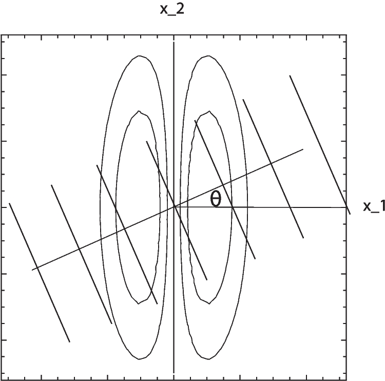
To quantify and visualize the characteristics and evolution of pathway formation, we construct several metrics described below. As the basic concept characterizing pathways is the consideration of excitatory synapses as vectors, \(\vec }\), with a magnitude equal to the value of the weight \(W_\) and direction defined by the orientation within our lattice of a vector originating at the excitatory presynaptic neuron i and ending at the postsynaptic neuron j. With this definition, we can readily quantify regional changes in the synaptic weights from the start to the end of a selected period \(\Delta t_\) by defining the average weight change vector \(\Delta \vec _s(\Delta t_)\) in region s by,

$$\begin \Delta \vec _s(\Delta t_) = \frac}}\sum _^s \Delta \vec }(\Delta t_) \end$$

(14)

where \(\Delta \vec _(\Delta t_)\) is the change in synaptic weight between neurons \(i'\) and \(j'\) over the same time period, and \(N_\) is the total number of excitatory synapses in the corresponding region s.

Comparison of the network activity and synaptic weights with and without plasticity. (a) shows network activity 70 ms after the \(i=100\) stimulation on a network without synaptic plasticity (\(R = 0\)). (b) shows network activity 70 ms after the \(i=100\) stimulation on a network with synaptic plasticity (\(R=4\)). The color of each (X, Y) position represents the average membrane potential v of the three lattice positions along the Z direction. Vector field of the average synaptic weights for each \(5\times 5\) region of the networks (excluding edge regions) after the \(i=100\) stimulation without STDP and with (\(R=4\)) STDP are shown in (c) and (d), respectively

To measure orientational order, we define an average local order parameter O that measures the degree of orientation between adjacent weight vectors and is given by,

$$\begin O = \left\langle \frac\sum _^ \langle \hat \rangle \cdot \langle \hat} \rangle \right\rangle _ \end$$

(15)

where \(\langle \hat \rangle \) is the unit vector in the direction of the average outgoing weight for neuron i, the domain of the sum nn is over the nearest neighborhood of i, and \(N'\) is the number of adjacent neurons to i. Operationally, O is calculated by first determining the \(\langle \hat \rangle \) unit vectors, then the sum of the dot products to all nearest neighbors \(j'\) is calculated, and finally this is averaged across the entire network as a measure of the average local order. The maximum value of this parameter is 1 if all unit average weight vectors point in the same direction, and the minimum is 0 for random orientations. To ameliorate edge effects resulting from our open boundary conditions, the neurons at the 2 outermost lattice positions in x and y are excluded from this calculation. Additionally, the z-component of vectors are excluded from this calculation for the same reason. An increase from zero of this parameter as a function of time will be an indication of the formation of synaptic pathways.

To measure the firing activity per neuron of the networks we calculate the firing rate of the whole neuronal population \(A(\Delta t_m)\) over a given measurement time period \(\Delta t_m = 100\) ms by using,

$$\begin A(\Delta t_m) = \frac(\Delta t_m)} \cdot \Delta t_m} \end$$

(16)

where \(N_\) is the total number of spikes in that time period normalized by \(N_\), the total number of neurons in the network.

For the particular case of the central stimulation experiment, we additionally measure the average radial propagation speed of the traveling wave front, v, given by,

$$\begin = \frac} \end$$

(17)

where \(\langle \Delta r\rangle \) is the average of the distances between the center of the stimulation and the location of the firing neurons after a chosen interval of \(\Delta t_ = 80\) ms following the stimulation event. While this measure takes into account all spikes regardless of their proximity to the wave front, the results are consistent and represent the corresponding traveling wave fronts because the number of spontaneously occurring spikes outside of the propagating wave is proportionally minuscule.

Visualization of network activity after applying central stimulation with \(R = 4\) for a single random seed. Successive snapshots show the network activity in 15ms intervals after (a) the first and (b) the hundredth central stimulation, respectively. The color of each (X, Y) position represents the average membrane potential v of the three lattice positions along the Z direction. vector fields of the average weight change for each \(5\times 5\) region for the first three central stimulations are shown in (c), equivalently scaled for comparison