In this section, we will theoretically analyze the orientation selectivity properties of the above described purely spatial as well as joint spatio-temporal models for receptive fields, when exposed to sine wave patterns with different orientations in relation to the preferred orientation of the receptive field.

4.1 Motivation for separate analyses for the different classes of purely spatial or joint spatio-temporal receptive field models, as well as motivation for studying the orientation selectivity curves for models of both simple cells and complex cells

A main reason for performing separate analyses for both purely spatial and joint spatio-temporal models, is that, a priori, it may not be clear how the results from an analysis of the orientation selectivity of a purely spatial model would relate to the results from an orientation selectivity analysis of a joint spatio-temporal model. Furthermore, within the domain of joint spatio-temporal models, it is not a priori clear how the results from an orientation selectivity analysis of a space-time separable spatio-temporal model would relate to the results for a velocity-adapted spatio-temporal model. For this reason, we will perform separate individual analyses for these three main classes of either purely spatial or joint spatio-temporal receptive field models.

Additionally, it may furthermore not be a priori clear how the results from orientation selectivity analyses of models of simple cells that have different numbers of dominant spatial or spatio-temporal lobes would relate to each other, nor how the results from an orientation selectivity analysis of a model of a complex cell would relate to the analysis of orientation selectivity of models of simple cells. For this reason, we will also perform separate analyses for models of simple and complex cells, for each one of the above three main classes of receptive field models, which leads to a total number of \((2 + 1) + (2 \times 2 + 1) + (2 + 1) = 11\) separate analyses, in the cases of either purely spatial, space-time separable or velocity-adapted receptive spatio-temporal fields, respectively, given that we restrict ourselves to simple cells that can be modelled in terms of either first- or second-order spatial and/or temporal derivatives of affine Gaussian kernels. The reason why there are \(2 \times 2 + 1 = 5\) subcases for the space-time separable spatio-temporal model is that we consider all the possible combinations of first- and second-order spatial derivatives with all possible combinations of first- and second-order temporal derivatives.

As will be demonstrated from the results, to be summarized in Table 1, the results from the orientation selectivity of the simple cells will turn out be similar within the class of purely first-order simple cells between the three classes of receptive field models (purely spatial, space-time separable or velocity-adapted spatio-temporal), as well as also similar within the class of purely second-order simple cells between the three classes of receptive field models. Regarding the models of complex cells, the results of the orientation selectivity analysis will be similar between the purely spatial and the velocity-adapted spatio-temporal receptive field models, whereas the results from the space-time separable spatio-temporal model of complex cells will differ from the other two. The resulting orientation selectivity curves will, however, differ between the sets of (i) first-order simple cells, (ii) second-order simple cells and (iii) complex cells.

The resulting special handling of the different cases that will arise from this analysis, with their different response characteristics, is particularly important, if one wants to fit parameterized models of orientation selectivity curves to actual neurophysiological data. If we want to relate neurophysiological findings measured for neurons, that are exposed to time-varying visual stimuli, or for neurons that have a strong dependency on temporal variations in the visual stimuli, then our motivation for performing a genuine spatio-temporal analysis for each one of the main classes of spatio-temporal models for simple cells, is to reduce the explanatory gap between the models and actual biological neurons.

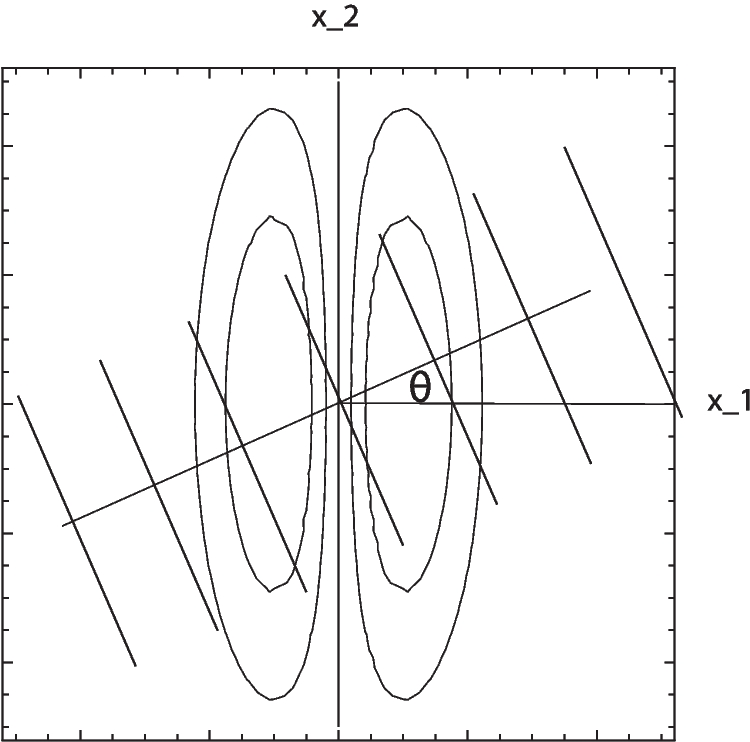
Table 1 Summary of the forms of the orientation selectivity functions derived from the theoretical models of simple cells and complex cells based on the generalized Gaussian derivative model for visual receptive fields, in the cases of either (i) purely spatial models, (ii) space-time separable spatio-temporal models and (iii) velocity-adapted spatio-temporal models4.2 Modelling scenario

For simplicity of analysis, and without loss of generality, we will henceforth align the coordinate system with the preferred orientation of the receptive field, in other words choosing the coordinate system such that the orientation angle \(\varphi = 0\). Then, we will expose this receptive field to static or moving sine wave patterns, that are oriented with respect to an inclination angle \(\theta \) relative to the resulting horizontal \(x_1\)-direction, as illustrated in Fig. 1. Figure 2 shows maps of the underlying first-order and second-order Gaussian derivatives for different degrees of elongation of the receptive fields.

Fig. 1

Schematic illustration of the modelling situation studied in the theoretical analysis, where the coordinate system is aligned to the preferred orientation \(\varphi = 0\) of the receptive field, and the receptive field is then exposed to a sine wave pattern with inclination angle \(\theta \). In this figure, the sine wave pattern is schematically illustrated by a set of level lines, overlayed onto a few level curves of a first-order affine Gaussian derivative kernel. (Horizontal axis: spatial coordinate \(x_1\). Vertical axis: spatial coordinate \(x_2\))

By necessity, the presentation that will follow will be somewhat technical, since we will analyze the properties of our mathematical models for the receptive fields of simple and complex cells for three different main cases of either (i) purely spatial receptive fields, (ii) space-time separable spatio-temporal receptive fields and (iii) velocity-adapted spatio-temporal receptive fields.

Readers, who may be more interested in the final results only and their biological implications, while not in the details of the mathematical modelling with its associated theoretical analysis, can without major loss of continuity proceed directly to Sect. 4.6, where a condensed overview is given of the derived orientation selectivity results.

Readers, who additionally is interested in getting just a brief overview of how the theoretical analysis is carried out, and the assumptions regarding the probing of the receptive fields that it rests upon, would be recommended to additionally read at least one of the theoretical modelling cases, where the purely spatial analysis in the following Sect. 4.3 then constitutes the simplest case.

Fig. 2

Affine Gaussian derivative receptive fields of orders 1 and 2 for the image orientation \(\varphi = 0\), with the scale parameter ratio \(\kappa = \sigma _2/\sigma _1\) increasing from 1 to \(4\sqrt\) according to a logarithmic distribution, from left to right, with the larger of these scale parameters \(\sigma _2\) kept constant. (top row) First-order directional derivatives of affine Gaussian kernels according to Eq. (1) for \(m = 1\). (bottom row) Second-order directional derivatives of affine Gaussian kernels according to Eq. (1) for \(m = 2\). (Horizontal axes: image coordinate \(x_1\). Vertical axes: image coordinate \(x_2\))

Fig. 3

Graphs of the orientation selectivity for purely spatial models of (left column) simple cells in terms of first-order directional derivatives of affine Gaussian kernels, (middle column) simple cells in terms of second-order directional derivatives of affine Gaussian kernels and (right column) complex cells in terms of directional quasi-quadrature measures that combine the first- and second-order simple cell responses in a Euclidean way for \(C = 1/\sqrt\), and shown for different values of the ratio \(\kappa \) between the spatial scale parameters in the vertical vs. the horizontal directions. Observe how the degree of orientation selectivity varies strongly depending on the eccentricity \(\epsilon = 1/\kappa \) of the receptive fields. (top row) Results for \(\kappa = 1\). (second row) Results for \(\kappa = 2\). (third row) Results for \(\kappa = 4\). (bottom row) Results for \(\kappa = 8\). (Horizontal axes: orientation \(\theta \in [-\pi /2, \pi /2]\). Vertical axes: Amplitude of the receptive field response relative to the maximum response obtained for \(\theta = 0\))

4.3 Analysis for purely spatial models of receptive fields

For the forthcoming purely spatial analysis, we will analyze the response properties of our spatial models of simple and complex cells to sine wave patterns with angular frequency \(\omega \) and orientation \(\theta \) of the form

$$\begin f(x_1, x_2) = \sin \left( \omega \cos (\theta ) \, x_1 + \omega \sin (\theta ) \, x_2+ \beta \right) . \end$$

(27)

4.3.1 First-order simple cell

Consider a simple cell that is modelled as a first-order scale-normalized derivative of an affine Gaussian kernel (according to Eq. (1) for \(m = 1\)), and oriented in the horizontal \(x_1\)-direction (for \(\varphi = 0\)) with spatial scale parameter \(\sigma _1\) in the horizontal \(x_1\)-direction and spatial scale parameter \(\sigma _2\) in the vertical \(x_2\)-direction, and thus a spatial covariance matrix of the form \(\varSigma _0 = \operatorname (\sigma _1^2, \sigma _2^2)\):

$$\begin &T_}(x_1, x_2;\; \sigma _1, \sigma _2) = \end}\nonumber \\ &= \frac \, \partial _ \left( e^ \right) \end}\nonumber \\ &= - \frac \, e^. \end} \end$$

(28)

The corresponding receptive field response is then, after solving the convolution integralFootnote 6 in Mathematica,

$$\begin L_}(x_1, x_2;\; \sigma _1, \sigma _2) = \end}\nonumber \\ &= \int _^ \int _^ T_}(\xi _1, \xi _2;\; \sigma _1, \sigma _2) \end}\nonumber \\ &} \times f(x_1 - \xi _1, x_2 - \xi _2) \, d \xi _1 \xi _2 \end}\nonumber \\ &= \omega \, \sigma _1 \cos (\theta ) \, e^ \omega ^2 (\sigma _1^2 \cos ^2 \theta + \sigma _2^2 \sin ^2 \theta )} \end}\nonumber \\ &} \times \cos ( \omega \cos (\theta ) \, x_1 + \omega \sin (\theta ) \, x_2+ \beta ), \end} \end$$

(29)

i.e., a cosine wave with amplitude

$$\begin A_(\theta , \omega ;\; \sigma _1, \sigma _2) = \omega \, \sigma _1 \left| \cos \theta \right| \, e^ \omega ^2 (\sigma _1^2 \cos ^2 \theta + \sigma _2^2 \sin ^2 \theta )}. \end$$

(30)

If we assume that the receptive field is fixed, then the amplitude of the response will depend strongly on the angular frequency \(\omega \) of the sine wave. The value first increases because of the factor \(\omega \) and then decreases because of the exponential decrease with \(\omega ^2\).

If we assume that a biological experiment regarding orientation selectivity is carried out in such a way that the angular frequency is varied for each inclination angle \(\theta \), and then that the result is for each value of \(\theta \) reported for the angular frequency \(\hat\) that leads to the maximum response, then we can determine this value of \(\hat\) by differentiating \(A_(\theta , \omega ;\; \sigma _1, \sigma _2)\) with respect to \(\omega \) and setting the derivative to zero, which gives:

$$\begin \hat_ = \frac}. \end$$

(31)

Inserting this value into \(A_(\theta , \omega ;\; \sigma _1, \sigma _2)\), and introducing a scale parameter ratio \(\kappa \) such that

$$\begin \sigma _2 = \kappa \, \sigma _1, \end$$

(32)

which implies

$$\begin \hat_ = \frac}, \end$$

(33)

then gives the following orientation selectivity measure

$$\begin A_(\theta , \; \kappa ) = \frac \sqrt}. \end$$

(34)

Note, specifically, that this amplitude measure is independent of the spatial scale parameter \(\sigma _1\) of the receptive field, which, in turn, is a consequence of the scale-invariant nature of differential expressions in terms of scale-normalized derivatives for scale normalization parameter \(\gamma = 1\).

The left column in Fig. 3 shows the result of plotting the measure \(A_(\theta ;\; \kappa )\) of the orientation selectivity as function of the inclination angle \(\theta \) for a few values of the scale parameter ratio \(\kappa \), with the values rescaled such that the peak value for each graph is equal to 1. As can be seen from the graphs, the degree of orientation selectivity increases strongly with the value of the spatial scale ratio parameter \(\kappa \).

4.3.2 Second-order simple cell

Consider next a simple cell that can be modelled as a second-order scale-normalized derivative of an affine Gaussian kernel (according to Eq. (1) for \(m = 2\)), and oriented in the horizontal \(x_1\)-direction (for \(\varphi = 0\)) with spatial scale parameter \(\sigma _1\) in the horizontal \(x_1\)-direction and spatial scale parameter \(\sigma _2\) in the vertical \(x_2\)-direction, and thus again with a spatial covariance matrix of the form \(\varSigma _0 = \operatorname (\sigma _1^2, \sigma _2^2)\):

$$\begin &T_}(x_1, x_2;\; \sigma _1, \sigma _2) = \end}\nonumber \\ &= \frac \, \partial _ \left( e^ \right) \end}\nonumber \\ &= \frac \, e^. \end} \end$$

(35)

The corresponding receptive field response is then, again after solving the convolution integral in Mathematica,

$$\begin L_}(x_1, x_2;\; \sigma _1, \sigma _2) = \end}\nonumber \\ &= \int _^ \int _^ T_}(\xi _1, \xi _2;\; \sigma _1, \sigma _2) \end}\nonumber \\ &} \times f(x_1 - \xi _1, x_2 - \xi _2) \, d \xi _1 \xi _2 \end}\nonumber \\ &= - \omega ^2 \, \sigma _1^2 \cos ^2 (\theta ) \, e^ \omega ^2 (\sigma _1^2 \cos ^2 \theta + \sigma _2^2 \sin ^2 \theta )} \end}\nonumber \\ &} \times \sin ( \omega \cos (\theta ) \, x_1 + \omega \sin (\theta ) \, x_2 + \beta ), \end} \end$$

(36)

i.e., a sine wave with amplitude

$$\begin&A_(\theta , \omega ;\; \sigma _1, \sigma _2)\nonumber \\&\quad = \omega ^2 \, \sigma _1^2 \cos ^2 (\theta ) \, e^ \omega ^2 (\sigma _1^2 \cos ^2 \theta + \sigma _2^2 \sin ^2 \theta )}. \end$$

(37)

Fig. 4

The expression for the oriented spatial quasi-quadrature measure \(\mathcal_,\text} L\) in the purely spatial model Eq. (40) of a complex cell, when applied to a sine wave pattern of the form Eq. (27), for \(\omega = \omega _\mathcal\) according to Eq. (41)

Again, also this expression first increases and then increases with the angular frequency \(\omega \). Selecting again the value of \(\hat\) at which the amplitude of the receptive field response assumes its maximum over \(\omega \) gives

$$\begin \hat_ = \frac}}, \end$$

(38)

and implies that the maximum amplitude over spatial scales as function of the inclination angle \(\theta \) and the scale parameter ratio \(\kappa \) can be written

$$\begin A_(\theta ;\; \kappa ) = \frac. \end$$

(39)

Again, this amplitude measure is also independent of the spatial scale parameter \(\sigma _1\) of the receptive field, because of the scale-invariant property of scale-normalized derivatives, when the scale normalization parameter \(\gamma \) is chosen as \(\gamma = 1\).

The middle column in Fig. 3 shows the result of plotting the measure \(A_(\theta ;\; \kappa )\) of the orientation selectivity as function of the inclination angle \(\theta \) for a few values of the scale parameter ratio \(\kappa \), with the values rescaled such that the peak value for each graph is equal to 1. Again, the degree of orientation selectivity increases strongly with the value of \(\kappa \), as for the first-order model of a simple cell.

4.3.3 Complex cell

To model the spatial response of a complex cell according to the spatial quasi-quadrature measure in Eq. (10), we combine the responses of the first- and second-order simple cells for \(\varGamma = 0\):

$$\begin \mathcal_,\text} L = \sqrt}^2 + C_ \, L_}^2}, \end$$

(40)

with \(L_}\) according to Eq. (29) and \(L_}\) according to Eq. (36). Choosing the angular frequency \(\hat\) as the geometric average of the angular frequencies for which the first- and second-order components of this entity assume their maxima over angular frequencies, respectively,

$$\begin \hat_\mathcal = \sqrt_ \, \hat_} = \frac}}, \end$$

(41)

with \(\hat_\) according to Eq. (33) and \(\hat_\) according to Eq. (38). Again letting \(\sigma _1 = \kappa \, \sigma _1\), and settingFootnote 7 the relative weight between first- and second-order information to \(C_ = 1/\sqrt\) according to Lindeberg (2018), gives the expression according to Eq. (26) in Fig. 4.

For inclination angle \(\theta = 0\), that measure is spatially constant, in agreement with previous work on closely related isotropic purely spatial isotropic quasi-quadrature measures (Lindeberg, 2018). Then, the spatial phase dependency increases with increasing values of the inclination angle \(\theta \). To select a single representative of those differing representations, let us choose the geometric average of the extreme values, which then assumes the form

$$\begin A_,\text}(\theta ;\; \kappa ) = \frac \, \left| \cos \theta \right| ^3} \left( \cos ^2 \theta + \kappa ^2 \sin ^2\theta \right) ^}. \end$$

(42)

The right column in Fig. 3 shows the result of plotting the measure \(A_,\text}(\theta ;\; \kappa )\) of the orientation selectivity as function of the inclination angle \(\theta \) for a few values of the scale parameter ratio \(\kappa \), with the values rescaled such that the peak value for each graph is equal to 1. As can be seen from the graphs, the degree of orientation selectivity increases strongly with the value of \(\kappa \) also for this model of a complex cell, and in a qualitatively similar way as for the simple cell models.

4.4 Analysis for space-time separable models of spatio-temporal receptive fields

To simplify the main flow through the paper, the detailed analysis of the orientation selectivity properties for the space-time separable models for the receptive fields of simple and complex cells is given in Appendix A.1, with the main results summarized in Sect. 4.6. Readers, who are mainly interested in understanding the principles by which the theoretical analysis is carried out, can proceed directly to Sect. 4.5, without major loss of continuity.

The main conceptual difference with the analysis of the space-time separable spatio-temporal receptive field models in Appendix A.1, compared to the purely spatial models in Sect. 4.3 or the velocity-adapted spatio-temporal receptive field models in Sect. 4.5, is that the space-time separable spatio-temporal receptive field models in Appendix A.1 do additionally involve derivatives with respect to time.

Fig. 5

Graphs of the orientation selectivity for velocity-adapted spatio-temporal models of (left column) simple cells in terms of first-order directional derivatives of affine Gaussian kernels combined with zero-order temporal Gaussian kernels, (middle column) simple cells in terms of second-order directional derivatives of affine Gaussian kernels combined with zero-order temporal Gaussian kernels and (right column) complex cells in terms of directional quasi-quadrature measures that combine the first- and second-order simple cell responses in a Euclidean way for \(C_ = 1/\sqrt\) shown for different values of the ratio \(\kappa \) between the spatial scale parameters in the vertical vs. the horizontal directions. Observe how the degree of orientation selectivity varies strongly depending on the eccentricity \(\epsilon = 1/\kappa \) of the receptive fields. (top row) Results for \(\kappa = 1\). (second row) Results for \(\kappa = 2\). (third row) Results for \(\kappa = 4\). (bottom row) Results for \(\kappa = 8\). (Horizontal axes: orientation \(\theta \in [-\pi /2, \pi /2]\). Vertical axes: Amplitude of the receptive field response relative to the maximum response obtained for \(\theta = 0\))

4.5 Analysis for velocity-adapted spatio-temporal models of receptive fields

Let us next analyze the response properties of non-separable velocity-adapted spatio-temporal receptive fields to a moving sine wave of the form

$$\begin f(x_1, x_2, t) = \\ = \sin \left( \omega \cos (\theta ) \, x_1 + \omega \sin (\theta ) \, x_2 - u \, t + \beta \right) . \end$$

(44)

Based on the observation that the response properties of temporal derivatives will be zero, if the (scalar) velocity v of the spatio-temporal receptive field model is adapted to the (scalar) velocity u of the moving sine wave, we will study the case when the temporal order of differentiation n is zero.

4.5.1 First-order simple cell

Consider a velocity-adapted receptive field corresponding to a first-order scale-normalized Gaussian derivative with scale parameter \(\sigma _1\) and velocity v in the horizontal \(x_1\)-direction, a zero-order Gaussian kernel with scale parameter \(\sigma _2\) in the vertical \(x_2\)-direction, and a zero-order Gaussian derivative with scale parameter \(\sigma _t\) in the temporal direction, corresponding to \(\varphi = 0\), \(v = 0\), \(\varSigma _0 = \operatorname (\sigma _1^2, \sigma _2^2)\), \(m = 1\) and \(n = 0\) in Eq. (13):

$$\begin &T_}(x_1, x_2, t;\; \sigma _1, \sigma _2, \sigma _t) = \end}\nonumber \\ &= \frac \, \sigma _1 \sigma _2 \sigma _t} \, \partial _ \left. \left( e^ \right) \right| _ \end}\nonumber \\ &= \frac \, \sigma _1^2 \sigma _2 \sigma _t} \, e^. \end} \end$$

(45)

The corresponding receptive field response is then, after solving the convolution integral in Mathematica,

$$\begin L_}(x_1, x_2, t;\; \sigma _1, \sigma _2, \sigma _t) = \end}\nonumber \\ &= \int _^ \int _^ \int _^ T_}(\xi _1, \xi _2, \zeta ;\; \sigma _1, \sigma _2, \sigma _t) \end}\nonumber \\ &} \times f(x_1 - \xi _1, x_2 - \xi _2, t - \zeta ) \, d \xi _1 \xi _2 d\zeta \end}\nonumber \\ &= \omega \, \sigma _1 \cos \theta \, \end}\nonumber \\ &} \times e^ \left( \left( \sigma _1^2+\sigma _t^2 v^2\right) \cos ^2 (\theta ) +\sigma _2^2 \sin ^2 \theta -2 \sigma _t^2 u v \cos \theta +\sigma _t^2 u^2\right) } \end}\nonumber \\ &} \times \cos \left( \cos (\theta ) \, x_1 + \sin (\theta ) \, x_2 -\omega \, u \, t + \beta \right) , \end} \end$$

(46)

i.e., a cosine wave with amplitude

$$\begin &A_(\theta , u, \omega ;\; \sigma _1, \sigma _2, \sigma _t) = \end}\nonumber \\ &= \omega \, \sigma _1 \left| \cos \theta \right| \, \end}\nonumber \\ &} \times e^ \left( \cos ^2 \theta \left( \sigma _1^2+\sigma _t^2 v^2\right) +\sigma _2^2 \sin ^2 \theta -2 \sigma _t^2 u v \cos \theta +\sigma _t^2 u^2\right) }. \end} \end$$

(47)

Assume that a biological experiment regarding the response properties of the receptive field is performed by varying both the angular frequency \(\omega \) and the image velocity u to get the maximum value of the response over these parameters. Differentiating the amplitude \(A_\) with respect to \(\omega \) and u and setting these derivatives to zero then gives

$$\begin \hat_ = \frac}, \end$$

(48)

$$\begin \hat_ = v \cos \theta . \end$$

(49)

Inserting these values into \(A_(\theta , u, \omega ;\; \sigma _1, \sigma _2, \sigma _t)\) then gives the following orientation selectivity measure

$$\begin A_(\theta , \; \kappa ) = \frac \, \sqrt}. \end$$

(50)

The left column in Fig. 5 shows the result of plotting the measure \(A_(\theta ;\; \kappa )\) of the orientation selectivity as function of the inclination angle \(\theta \) for a few values of the scale parameter ratio \(\kappa \), with the values rescaled such that the peak value for each graph is equal to 1. As we can see from the graphs, as for the previous purely spatial models of the receptive fields, as well as for the previous space-time separable model of the receptive fields, the degree of orientation selectivity increases strongly with the value of \(\kappa \).

4.5.2 Second-order simple cell

Consider next a velocity-adapted receptive field corresponding to a second-order scale-normalized Gaussian derivative with scale parameter \(\sigma _1\) and velocity v in the horizontal \(x_1\)-direction, a zero-order Gaussian kernel with scale parameter \(\sigma _2\) in the vertical \(x_2\)-direction, and a zero-order Gaussian derivative with scale parameter \(\sigma _t\) in the temporal direction, corresponding to \(\varphi = 0\), \(v = 0\), \(\varSigma _0 = \operatorname (\sigma _1^2, \sigma _2^2)\), \(m = 2\) and \(n = 0\) in Eq. (13):

$$\begin &T_}(x_1, x_2, t;\; \sigma _1, \sigma _2, \sigma _t) = \end}\nonumber \\ &= \frac \, \sigma _1 \sigma _2 \sigma _t} \, \partial _ \left. \left( e^ \right) \right| _ \end}\nonumber \\ &= \frac \, \sigma _1^3 \sigma _2 \sigma _t} \, e^. \end} \end$$

(51)

Fig. 6

The expression for the oriented spatio-temporal quasi-quadrature measure \(\mathcal_,\text} L\) in the velocity-adapted spatio-temporal model Eq. (23) of a complex cell, when applied to a sine wave pattern of the form Eq. (44), for \(\omega = \omega _\mathcal\) according to Eq. (58) and \(u = u_\mathcal\) according to Eq. (59)

The corresponding receptive field response is then, after solving the convolution integral in Mathematica,

$$\begin L_}(x_1, x_2, t;\; \sigma _1, \sigma _2, \sigma _t) = \end}\nonumber \\ &= \int _^ \int _^ \int _^ T_}(\xi _1, \xi _2, \zeta ;\; \sigma _1, \sigma _2, \sigma _t) \end}\nonumber \\ &} \times f(x_1 - \xi _1, x_2 - \xi _2, t - \zeta ) \, d \xi _1 \xi _2 d\zeta \end}\nonumber \\ &= -\omega ^2 \sigma _1^2 \cos ^2 \theta \, \end}\nonumber \\ &} \times e^ \left( \left( \sigma _1^2+\sigma _t^2 v^2\right) \cos ^2 \theta +\sigma _2^2 \sin ^2 \theta -2 \sigma _t^2 u v \cos \theta +\sigma _t^2 u^2\right) } \end}\nonumber \\ &} \times \cos \left( \sin (\theta ) \, x_1 + \sin (\theta ) \, x_2 - \omega \, u \, t + \beta \right) , \end} \end$$

(52)

i.e., a sine wave with amplitude

$$\begin & A_(\theta , u, \omega ;\; \sigma _1, \sigma _2, \sigma _t) = \\ \end}\nonumber \\ &= \omega ^2 \sigma _1^2 \cos ^2 \theta \, \end}\nonumber \\ &} \times e^ \left( \cos ^2 \theta \left( \sigma _1^2+\sigma _t^2 v^2\right) +\sigma _2^2 \sin ^2 \theta -2 \sigma _t^2 u v \cos \theta +\sigma _t^2 u^2\right) }. \end} \end$$

(53)

Assume that a biological experiment regarding the response properties of the receptive field is performed by varying both the angular frequency \(\omega \) and the image velocity u to get the maximum value of the response over these parameters. Differentiating the amplitude \(A_\) with respect to \(\omega \) and u and setting these derivatives to zero then gives

$$\begin \hat_ = \frac}}, \end$$

(54)

$$\begin \hat_ = v \cos \theta . \end$$

(55)

Inserting these values into \(A_(\theta , u, \omega ;\; \sigma _1, \sigma _2, \sigma _t)\) then gives the following orientation selectivity measure

$$\begin A_(\theta , \; \kappa ) = \frac. \end$$

(56)

The middle column in Fig. 5 shows the result of plotting the measure \(A_(\theta ;\; \kappa )\) of the orientation selectivity as function of the inclination angle \(\theta \) for a few values of the scale parameter ratio \(\kappa \), with the values rescaled such that the peak value for each graph is equal to 1. Again, the degree of orientation selectivity increases strongly with the value of \(\kappa \).

4.5.3 Complex cell

To model the spatial response of a complex cell according to the spatio-temporal quasi-quadrature measure Eq. (23) based on velocity-adapted spatio-temporal receptive fields, we combine the responses of the first- and second-order simple cells (for \(\varGamma = 0\))

$$\begin (\mathcal_,\text} L) = \sqrt}^2 + \, C_ \, L_}^2}^}}, \end$$

(57)

with \(L_}\) according to Eq. (46) and \(L_}\) according to Eq. (52).

Selecting the angular frequency as the geometric average of the angular frequency values at which the above spatio-temporal simple cell models assume their maxima over angular frequencies, as well as using the same value of u,

$$\begin \hat_\mathcal = \sqrt_ \, \hat_} = \frac}}, \end$$

(58)

with \(\hat_\) according to Eq. (48) and \(\hat_\) according to Eq. (54), as well as choosing the image velocity \(\hat\) as the same value as for which the above spatio-temporal simple cell models assume their maxima over the image velocity (Eqs. (49) and (55))

$$\begin \hat_\mathcal = v \cos \theta , \end$$

(59)

as well as letting \(\sigma _1 = \kappa \, \sigma _1\), and setting the relative weights between first- and second-order information to \(C_ = 1/\sqrt\) and \(C_t = 1/\sqrt\) according to Lindeberg (2018), then gives the expression according to Eq. (43) in Fig. 6.

For inclination angle \(\theta = 0\), that measure is spatially constant, in agreement with our previous purely spatial analysis, as well as in agreement with previous work on closely related isotropic spatio-temporal quasi-quadrature measures (Lindeberg, 2018). When the inclination angle increases, the phase dependency of the quasi-quadrature measure will, however, increase. To select a single representative of those differing representations, let us choose the geometric average of the extreme values, which then assumes the form

$$\begin A_,\text,\max }(\theta ;\; \kappa ) = \frac \, \left| \cos \theta \right| ^ }} \, (\cos ^2 \theta + \kappa ^2 \sin ^2\theta )^}. \end$$

(60)

The right column in Fig. 5 shows the result of plotting the measure \(A_,\text,\max }(\theta ;\; \kappa )\) of the orientation selectivity as function of the inclination angle \(\theta \) for a few values of the scale parameter ratio \(\kappa \), with the values rescaled such that the peak value for each graph is equal to 1. Again, the degree of orientation selectivity increases strongly with the value of \(\kappa \).

4.6 Resulting models for orientation selectivity

Table 1 summarizes the results from the above theoretical analysis of the orientation selectivity for our idealized models of simple cells and complex cells, based on the generalized Gaussian derivative model for visual receptive fields, in the cases of either (i) purely spatial models, (ii) space-time separable spatio-temporal models and (iii) velocity-adapted spatio-temporal models. The overall methodology that we have used for deriving these results is by exposing each theoretical receptive field model to either purely spatial or joint spatio-temporal sine wave patterns, and measuring the response properties for different inclination angles \(\theta \), at the angular frequency of the sine wave, as well as the image velocity of the spatio-temporal sine wave, at which these models assume their maximum response over variations of these probing parameters.

As can be seen from the table, the form of the orientation selectivity curve is similar for all the models of first-order simple cells, which correspond to first-order derivatives of affine Gaussian kernels over the spatial domain. The form of the orientation selectivity curve is also similar for all the models of second-order simple cells, which correspond to second-order derivatives of affine Gaussian kernels over the spatial domain. For complex cells, the form of the orientation selectivity curve for the space-time separable model is, however, different from the form of the orientation selectivity curve for the purely spatial model and the velocity-adapted spatio-temporal model, which both have a similar form for their orientation selectivity curves.

Note, in particular, that common for all these models is the fact that the degree of orientation selectivity increases with the scale parameter ratio \(\kappa = \sigma _2/\sigma _1\), which is the ratio between the scale parameter \(\sigma _2\) in the direction \(\bot \varphi \) perpendicular to the preferred orientation \(\varphi \) of the receptive field and the scale parameter \(\sigma _1\) in the preferred orientation \(\varphi \) of the receptive field. In other words, for higher values of \(\kappa \), the form of the orientation selectivity curve is more narrow than the form of the orientation selectivity curve for a lower value of \(\kappa \). The form of the orientation selectivity curve is also more narrow for a simple cell that can be modelled as a second-order directional derivative of an affine Gaussian kernel, than for a simple cell that can be modelled as a first order derivative of an affine Gaussian kernel.

In this respect, the theoretical analysis supports the conclusion that the degree of orientation selectivity of the receptive fields increases with the degree of anisotropy or elongation of the receptive fields, specifically the fact that highly anisotropic or elongated affine Gaussian derivative based receptive fields have higher degree of orientation selectivity than more isotropic affine Gaussian derivative based receptive fields.

The shapes of the resulting orientation selectivity curves do, however, notably differ between the classes of (i) first-order simple cells, (ii) second-order simple cells and (iii) complex cells. This property is important to take into account, if one aims at fitting parameterized models of orientation selectivity curves to neurophysiological measurements of corresponding data.