Participants and ethics statement

Participants were recruited in two separate studies (see below). The non-interventional study was approved by the local ethics committee (MSD-IDREC-C2-2014-023) and the interventional study by the National Research Ethics Service Committee South Central – Oxford A (15/SC/0109) and the Oxford Health NHS Foundation Trust. Participants gave informed consent and were reimbursed for taking part in the study. All methods were performed in accordance with the relevant guidelines and regulations.

Volunteers at suspected high vs low risk of bipolar disorder

Participants were recruited through local advertisement and from pools of previous participants. In an online pre-screening session, participants completed the Mood Disorders Questionnaire (MDQ [20]), a self-report screening instrument to identify risk for bipolar disorder. Participants were only invited for a full screening session if they scored either <5 points (‘low MDQ’ group, n = 37 included, at presumed low risk for bipolar disorder); or ≥7 (‘high MDQ’ group, n = 40 included). The screening verified that several of these symptoms measured with the MDQ happened during the same period of time. Structured clinical interviews with the SCID revealed that 5 of this group met criteria for bipolar disorder, despite not having received a formal diagnosis or seeking treatment. See Supplementary Method [1A] for detailed exclusion criteria.

Patients with BD

Participants were recruited through the BD Research Clinic (Oxford). All participants met criteria for BD-I (n = 7), BD-II (n = 27) or BD not otherwise specified (BD-NOS, n = 1), based on structured clinical interview. All participants were outside major mood episodes requiring immediate treatment. Full exclusion criteria are provided in the Supplementary Materials [1B]. Participants were assigned to placebo (n = 16) or lithium (n = 19), in a randomised double-blind design, see below.

Study designVolunteers

We measured participants’ mood and behaviour in a cognitive task longitudinally five times a week over ten weeks. Brain activity during the same task was measured during an MRI scan. The data here were part of a larger study (Supplementary Method [1B]).

Patients with BD

This study was a randomised, 6-week, double-blind, placebo-controlled trial [21]. See Supplementary Method [1B] for full information. All participants underwent a two-week pre-randomization phase (‘baseline’) during which they completed the cognitive task and mood ratings daily at home. Due to logistic challenges, for some participants this phase lasted longer than two weeks. For the next phase (6 weeks), participants were pseudo-randomly assigned to receive either lithium (starting dose of 400 mg and then titrated to plasma levels of 0.6–1 mmol/L) or placebo in a double-blind design. Only 22 participants were fMRI compatible. Participants were invited to complete online weekly assessments of depression symptoms with the Quick Inventory of Depressive Symptomatology (QIDS, [22]) and symptoms of Mania with the Altman Self Rating Mania Scale [23].

Throughout, we performed two types of group comparisons. First, we compared across risk of BD (i.e. group as ordered factor [24] in regressions, Low MDQ ≤ High MDQ ≤ patients with BD), subsequently referred to as ‘bipolar disorder gradient’. Ordered factors in regression imply a relationship of order between the groups, this does not have to be a linear relationship (i.e. the difference low MDQ to high MDQ can be larger or smaller [but of same sign] than the difference high MDQ to patients with BD). MDQ was not measured in the patient group. As this involved data from the BD group before assignment to lithium or placebo, all participants were included. Significant results were post-hoc followed up comparisons of the individual groups (t-tests). Second, we tested for the effects of lithium treatment as drug (lithium/placebo) x time point (pre, i.e. baseline/post) interactions.

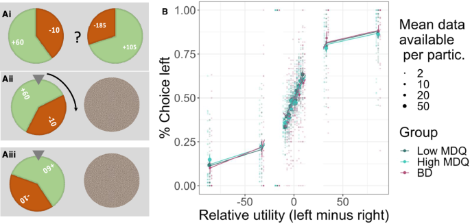
‘Wheel of fortune’ taskTrial structure

On each trial of the task, participants were given two options shown side-by-side. In the at-home version, these were wheels of fortune (Fig. 1A). In the fMRI version, they were instead presented as bars. Each option had three attributes: probability of winning vs. losing (size of green vs. red area), magnitude of possible gain (number on green area, 10–200), and magnitude of possible loss (number on red area, also 10–200). After participants chose one option, the wheel of fortune started spinning and then randomly landed on either win or loss. Finally, participants were shown their updated total score. The experiment was designed so that most choices were difficult, i.e., the options were very similar in expected value, i.e. relative utility (reward magnitude * probability; 90% of choices were not more than 20 points apart; 76% not more than 5 points apart, Fig. 1B, Supplementary Fig. S1).

Fig. 1: Task design and longitudinal behaviour.

A On each trial, participants chose between two gambles (‘wheel of fortune’) that differed in their probability of winning or losing points and in the number of points that could be won or lost. Once participants had chosen an option, the alternative was hidden, and the chosen wheel started spinning until finally landing on the win or loss. B Participants’ choices (left vs. right option) were guided by the relative utilities (reward utility – i.e., probability * magnitude – minus loss utility): the higher the utility of the left option, the more it was chosen. The computational model (lines) captured behaviour (dots with error bars) well. Data were combined across all testing sessions (up to 50) per participant (20 trials per session). Error bars show the standard error of the mean, and the size of the dots indicates the number of data points available.

Timings and number of trials

Each day, participants rated their positive and negative mood using the Positive and Negative Affect Schedule – Short Form, PANAS-SF [25]. They also gave an overall rating of their mood (‘How are you feeling’, referred to here as ‘happiness VAS’) using a slider ranging from ‘very unhappy’ (red sad face drawing) to ‘very happy’ (green smiley face). They then played 20 trials of the task. After the task, they repeated the happiness VAS.

In the fMRI scanner, participants played 100 trials. All timings were jittered. From the onset of options until participants could make a choice: 1–2 s; delay between participants’ response and outcomes shown: 2.7 to 7.7 s; duration of outcome shown: 1–3 s; duration of total score shown: 1–9 s; ITI: 1–9 s.

Behaviour

Behavioural data were analysed in R [26] (version 4.0.2) and Matlab. R-packages: Stan [27], BRMS [28, 29], dplyr [30], ggpubr [31], sjPlot [32], compareGroups [33], emmeans [34], ggsci [35].

Group comparisons

To compare groups, instead of a standard ANOVA procedure which tests for any differences between groups, we tested for a systematic effect, i.e. bipolar disorder gradient (group as ordered factor [24], Low MDQ ≤ High MDQ ≤ patients with BD) in linear regressions, also controlling for age and gender. Models used the BRMS toolbox interface for Stan (Supplementary Methods 2). For this and all subsequent analyses, we used Bayesian Credible Intervals [36] to establish significance by the 95% CI not including zero.

Computational modelsDecision making

We used a computational model to capture participants’ choices. The model first computed the overall expected value (‘utility’) of each option, then made a choice (left or right option) depending on which option had the better utility, but also allowing for some random choice behaviour [37, 38].

First, the model compared the options’ utilities as displayed at the time of choice on the current trial, i.e., probability (prob) x magnitude (mag). We allowed for individual differences in sensitivity to the loss vs. reward utility (λ). We also included in the model a measure of adaptions of risk taking (i.e. loss vs win sensitivity) to past outcomes (‘outcome history’). Specifically, a parameter (γ) changed the weighting of the loss utility on the current trial depending on whether the previous trial’s outcome was a win or a loss (i.e., γ > 0 means increased sensitivity to losses after a win on the previous trial).

$$}_}=* }_}-\left(}}}+}}}* }_}}}\right)* \left(1-\right)* }_}$$

To decide which option to choose, the model compared the utilities of the left and right options taking into account each participant’s ‘randomness’ (inverse temperature (β), higher numbers indicating higher choice consistency):

$$p\left(}_}\right)=\frac^}}}* (}_}-}_})}}$$

To allow fitting of individual sessions (20 trials), a Bayesian approach was implemented that allowed specifying priors for each parameter (Supplementary Methods [2C]). The model was validated using simulations and model comparisons (Supplementary Tables S1–3 and Supplementary Methods [2A–B]).

Group differences

To assess group differences, we entered the session-wise parameters into hierarchical regressions (using BRMS). This allowed us to take into account that parameters might change over days of testing, as well as individual differences in the means and variability (standard deviation) across sessions. For example:

Mean: invTemp(β) ~ 1 + day + group + Age + Gender + (1 + day | ID),

And error term: sigma ~ 1 + group + Age + Gender + (1|ID))

The effect of lithium (vs. placebo) was tested analogously:

Mean: invTemp(β) ~ 1 + day + group*pre, i.e. baseline/post + Age +Gender + number_days_baseline + (1 + day | ID)

These models were used for group comparisons of mean parameters (Supplementary Methods 2C, D). Variabilities of parameters over days were not compared as model validation (Supplementary Table S1) suggested poor recovery. Mood data (positive and negative PANAS, happiness VAS) were analysed using similar regressions (Supplementary Methods 2D) to assess group differences in mood (mean or variability) or the relationship between task outcomes and changes in happiness VAS.

Model-free analyses of behaviour

To test that participants could perform the task, i.e., that their choices were sensitive to expected value, we binned their choices (% left vs. right option) according to the overall utility difference between the two options (i.e., left vs. right reward utility minus loss utility, utility = probability*magnitude).

To test sensitivity to risk of losses, as has been previously reported to be affected in BD [39, 40], we refined the binning of choices (as above) by further splitting the data according to win and loss utility (i.e. probability * magnitude).

We next analysed behaviour for adaptions of risk taking to past outcomes by considering how participants change their behaviour – here risk-taking (avoidance of potential losses) – based on win/loss outcomes on previous trials (‘outcome history’ effect). For this, we computed how their choices differed after a win or loss on the previous trial (difference % choosing option with lower potential loss [loss utility] after win minus after a loss). We focused on the most extreme (lowest/highest) loss utility bins from the analyses above (‘taking loss utility more into account’) as adaptation to past trial outcomes by taking loss more into account (i.e. a multiplicative effect) should most strongly affect choices the more dissimilar the loss utilities of the two options.

MRI acquisition

Data from all 77 high and low MDQ volunteers and 13 patients with BD were collected on a 3T Siemens Magneton Trio. Data from 9 patients with BD were collected at a different site using a Siemens Magneton PRISMA. Group comparisons include scanner as a control regressor. Scan protocols were carried out following [14], Supplementary Methods [3A].

FMRI analysis – whole-brainGeneral approach

Data were pre-processed using FSL ([41], Supplementary Methods [3B]). Statistical analysis was performed at two levels, event-related GLM for each participant, followed by group-level mixed-effect model using FSL’s FLAME 1 [42, 43] with outlier de-weighting. Whole-brain images are all cluster-corrected (p < 0.05 two-tailed, FWE), voxel inclusion threshold: z < 2.3.

Regression designs

At the time of the decision, we looked for neural activity correlating with the utility (reward, loss) of the choice. At the time of the outcome of the gamble, we looked for neural activity related to the processing of the outcome (win/loss as continuous regressor). Decision and outcome-related activity could be dissociated due to jitter used in the experimental timing [14]. As a key measure of interest, we looked at whether there was a history effect at the time of the choice (i.e., previous trial’s gamble win/loss outcome [14, 44], analogous to the behavioural analyses). Full design information: Supplementary Methods [3C], Supplementary Fig. S2.

Group-level comparisons

We compared the low vs high MDQ groups (n = 77) in whole-brain analyses. As only 22 patients with BD were available, these group comparisons were first performed in regions of interest (ROIs) derived from comparisons of the high/low MDQ groups. As exploratory analyses, BD groups were also compared at the whole-brain level.

ROI analyses

Mean brain activations (COPES, contrasts of parameter estimates) were extracted for each participant. These were used to illustrate group differences and also to perform independent statistical tests (e.g., ROIs of clusters defined based on group differences of high vs. low MDQ could be used to test group differences between lithium and placebo). For this, non-hierarchical Bayesian regressions were used, also controlling for age and gender. Brain activations for the outcome history effect were correlated with the corresponding behavioural measures. For this, effects of age, gender and group (and for the patients with BD: number of days in the baseline phase pre-randomization, i.e. before the MRI scan) were first removed using regressions from both neural and behavioural measures.