This section details the components of the proposed CCL-ASPS. The utilized dataset and data preprocessing are presented first. Subsequently, the components of CCL-ASPS are introduced: graph structure-based feature extraction, collaborative contrastive learning with adaptive self-paced sampling, and the final predictor. The source code and dataset for CCL-ASPS are publicly available at 10.5281/zenodo.13329691.

Dataset and preprocessing

This study validates all innovations with one drug-target interaction dataset collected from multiple data sources. Interaction networks related to drugs and proteins are obtained from Luo [17]. SMILES strings of drugs are collected from DrugBank [47]. Protein amino acid sequences are retrieved from Uniport [48]. Protein 3D structures are acquired from the RCSB Protein Data Bank [49]. For proteins lacking PDB structures, predicted structures from AlphaFold [50] are utilized. As shown in Table 8, the final dataset contains 12015 nodes, including 708 drugs, 1512 proteins, 5603 diseases, and 4192 side effects. Furthermore, six types of interactions are collected, including 1923 drug-protein interactions (Dr-Pr), 199214 drug-disease associations (Dr-Di), 10036 drug-drug interactions (Dr-Dr), 80164 drug-side-effect associations (Dr-Se), 1923 protein-drug interactions (Pr-Dr), 1596745 protein-disease associations (Pr-Di), and 7363 protein-protein interactions (Pr-Pr).

Table 8 Statistics of the collected data

Afterward, the drug SMILES strings are converted into atom interaction graphs. Each atom feature is initialized based on its chemical properties [51]. For proteins, the coordinates of amino acid residues are represented by their \(C_\) atoms. The distances between residues are calculated. Residues are considered in contact if their distance is below a specified threshold, which forms the amino acid residue interaction graphs. Additionally, seven attributes of amino acid residues are utilized for initial representations [52].

Jaccard similarity [53] is employed to construct similarity networks based on each interaction and association network. Additionally, structure similarity networks are built based on SMILES strings and amino acid sequences using methods described in Luo [17].

Drug graph structure-based feature

This section describes the extraction of drug representations from atom interaction graphs using Graph Convolutional Network (GCN) [37].

For each drug \(d_i\), its initial atom representations are denoted as \(X_ \in \mathbb ^}\times k_}\), where \(n_}\) and \(k_\) represents the number of atoms in drug \(d_\) and the feature dimension of atoms, respectively. Additionally, matrix \(A_} \in \mathbb ^}\times n_}}\) denotes the adjacency matrix between atoms, where \(A_}=1\) means there is an edge between two atoms and \(A_}=0\) otherwise.

GCN updates the atom features by aggregating information from neighboring atoms, as defined by the following equation:

$$\begin X_^\prime =\sigma \left( D_}^} \check_} D_}^} X_ W_}\right) , \end$$

(1)

where \(\check_} = A_} + I\) is the adjacency matrix with self-loop, \(I\in \mathbb ^}\times n_}}\) is the identity matrix, \(D_} \in \mathbb ^}\times n_}}\) is the degree matrix with the value of each diagonal element equal to the degree of the corresponding atom node, \(W_} \in \mathbb ^ \times f_}\) is a learnable weight parameter and \(f_\) is the output feature dimension of atoms, \(\sigma \left( \cdot \right)\) is the nonlinear activation function.

Following the update of features, a readout function is employed to combine all the atom features and generate the drug representation.

$$\begin h_ =\left( X_^\prime \right) , \end$$

(2)

where \(h_ \in \mathbb ^}\) is the representation of drug \(d_i\). In this study, all \(\) functions are implemented using the global mean pooling operation.

To pre-train the GCN for drug feature extraction, a binary cross-entropy loss (BCELoss) is employed as the objective function, aiming to predict drug-drug interactions. This involves learning the joint representations of the drug-drug pairs with a CNN layer:

$$\begin } = \left( \left( h_\Vert h_\right) \right) , \end$$

(3)

where \(h_\) and \(h_\) are the representations of drug \(d_\) and \(d_\), respectively. The symbol \(\Vert\) denotes the concatenation operation. \(\) represents the CNN layer with a kernel size of 3, an out channel of 4, padding and step size of 1. \(\) represents the max pooling operation. The resulting \(\in \mathbb ^}}\) is the joint representation of drug \(d_\) and \(d_\).

A multilayer perceptron is applied to predict the association probability of drug pairs:

$$\begin } =\sigma \left( W_} \left( \left( W_} }\right) \right) \right) , \end$$

(4)

where \(W_} \in \mathbb ^ \times f_}\) and \(W_} \in \mathbb ^ \times 1}\) are learnable parameters, \(\sigma \left( \cdot \right)\) and \(\) are nonlinear activation functions, and \(}\) is the predicted association probability between drug \(d_i\) and \(d_j\).

The BCELoss serves as the objective function for drug feature extraction:

$$\begin \mathcal _ =-\sum \limits _ _} \log _} + (1-_}) \log (1-}), \end$$

(5)

where ddp denotes a set of drug-drug pairs. \((d_i,d_j)\) represents a single pair of drug \(d_i\) and \(d_j\). \(}\) represents the predicted association probability of drug pair \((d_i,d_j)\). \(_}\) signifies the ground truth for drug-drug association, where \(_=1}\) for true drug-drug association and \(_=0}\) otherwise.

Protein graph structure-based feature

Similar to drug feature extraction, a GCN-based approach is employed to extract protein features from the amino acid residue interaction graphs. The amino acid residue interaction graph for protein \(p_i\) is represented by an adjacency matrix \(A_ \in \mathbb ^\times n_}\), where \(n_\) denotes the number of residues in the protein \(p_i\). Each row in the initial feature matrix \(X_ \in \mathbb ^\times k_}\) represents the initial features of an amino acid residue. \(k_\) is the initial feature dimension of proteins.

A single-layer GCN is applied to update the residue representations, aggregating information from neighboring residues:

$$\begin X_^\prime =\left( \ W_ \left( D^}_ (A_ + I_) D^}_ X_ W_}\right) \right) , \end$$

(6)

where \(I_ \in \mathbb ^\times n_}\) is the identity matrix. \(D_ \in \mathbb ^\times n_}\) is a diagonal matrix with the corresponding values are nodes degree. \(W_}\in \mathbb ^ \times f_}\) and \(W_}\in \mathbb ^ \times f_}\) are learnable parameters. \(f_\) is the output feature dimension of amino acid residue. \(ReLu\left( \cdot \right)\) is an activation function. \(X_^\prime \in \mathbb ^\times f_}\) is the updated amino acid residue feature matrix.

Following the update, a self-attention pooling layer is employed to extract feature representations of key residues. Subsequently, a readout function is applied to obtain the protein representation for downstream tasks:

$$\begin h_ =\left( \left( X_^\prime \right) \right) , \end$$

(7)

where \(SAGPooling\left( \cdot \right)\) is the self-attention pooling. \(h_\in \mathbb ^}\) is the representation of protein \(p_i\).

To pre-train the GCN for protein feature extraction, the binary cross-entropy loss is applied as the objective function, aiming to predict protein-protein interactions (PPIs). The pre-training process is analogous to drug feature extraction. The implementation is the same as in Eqs. (3, 4, 5):

$$\begin } =\left( \left( h_\Vert h_\right) \right) , \end$$

(8)

$$\begin } =\sigma \left( W_} \left( W_} }\right) \right) , \end$$

(9)

$$\begin \mathcal _ =-\sum \limits _ _} \log _} + (1-_}) \log (1-}), \end$$

(10)

where \(h_\) and \(h_\) are representations of protein \(p_i\) and \(p_j\), respectively. \(h_}\in \mathbb ^}\) is the joint representation of protein \(p_i\) and \(p_j\). \(W_} \in \mathbb ^ \times f_}\) and \(W_} \in \mathbb ^ \times f_}\) are learnable parameters. \(}\) is the predicted interaction probability between protein \(p_i\) and \(p_j\). \(_}\) is the ground truth, with \(_=1}\) indicating an interaction between two proteins and \(_=0}\) otherwise.

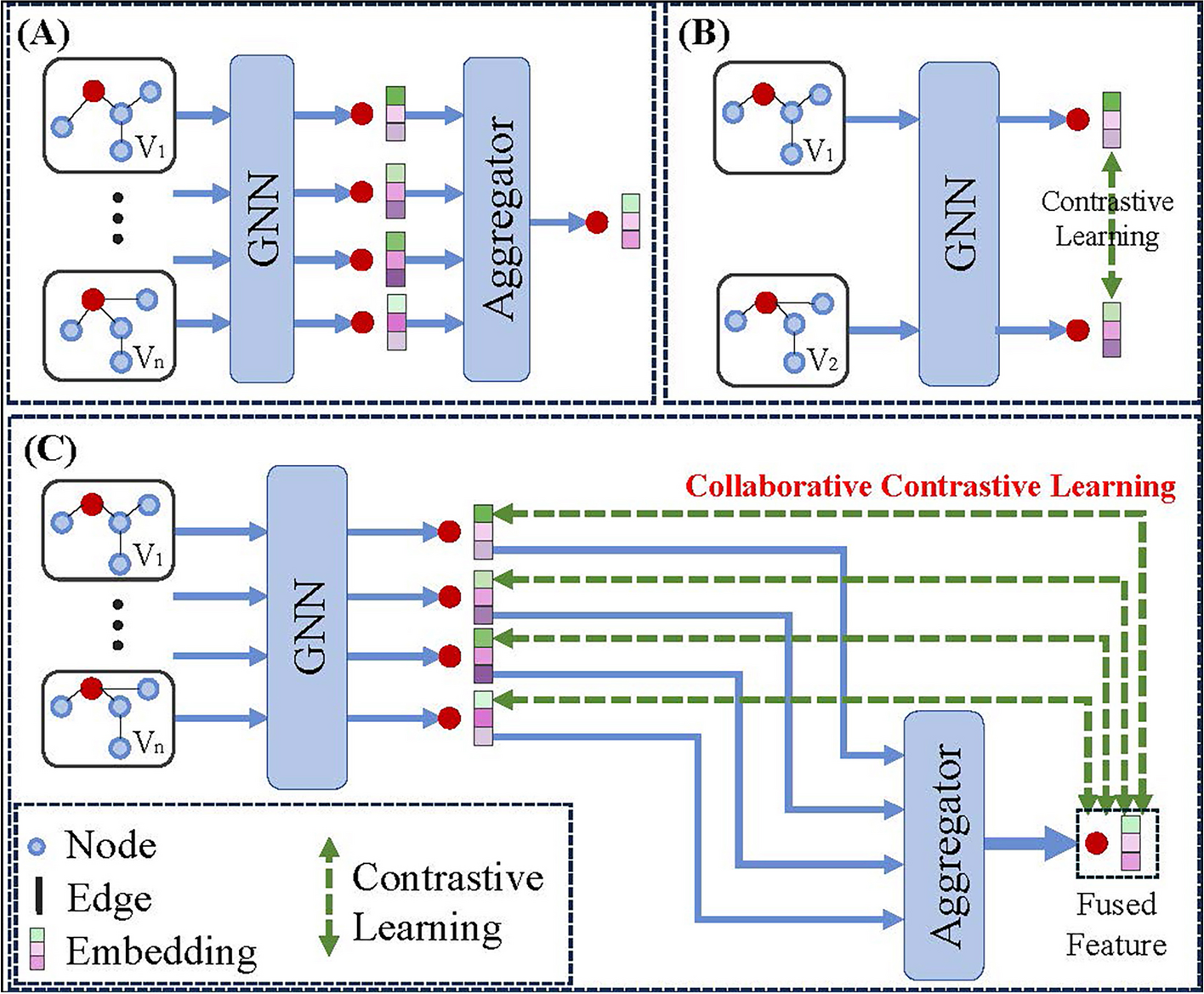
Collaborative contrastive learning with adaptive self-paced sampling

This section describes the proposed collaborative contrastive learning and adaptive self-paced sampling strategy, illustrated in Fig. 2B and C. The strategy consists of three key components: multiple network learning, collaborative contrastive learning, and adaptive self-paced sampling. The overall workflow is outlined in Algorithm 1.

Multiple network learning

This section introduces the first component: multiple network learning. GAT [38] is employed to leverage information hidden within each drug and protein similarity network.

With each similarity network \(S^m,\left( m=1,2,\ldots , n_\right)\), for each drug \(d_i\) and its pre-trained representation \(h_\), GAT computes normalized attention scores to its neighbors. The attention score \(\mathcal ^_\) for neighbor \(d_j\) at layer l is calculated as:

$$\begin \mathcal ^_ = \left( \frac_}} \in \mathcal (i)} e^_}\right) , \end$$

(11)

where \(e^_\) is the unnormalized attention score between drug \(d_i\) and \(d_j\) at layer l. \(\mathcal (i)\) denotes the set neighbors for drug \(d_i\).

The unnormalized attention score \(e^_\) is defined as:

$$\begin e^_ = ^\left( ( W^_1 h^_ \Vert W^_2 h^_) \right) , \end$$

(12)

where \(W^_1 \in \mathbb ^\times f_}\) and \(W^_2 \in \mathbb ^\times f_}\) are learnable weight matrices at layer l. \(} \in \mathbb ^}\) is a learnable parameter vector at layer l.

After computing the normalized attention scores \(\mathcal ^_\) for all neighbors, the GAT layer aggregates the features of neighboring drugs in a weighted manner to update the representation of the target drug \(d_i\):

$$\begin h^_ =\sigma \left( \sum \limits _(i)}_ W^_3 h^_} \right) , \end$$

(13)

where \(h^_\) denotes the output representation at layer l, with \(h^_ = h_\). \(W^_3 \in \mathbb ^\times f_}\) is the weight matrix in layer l.

The output of the final layer is considered the final representation learned from the similarity network \(S^m\), denoted as \(h^_\).

Similar to drug representation learning, protein features can be extracted from each protein similarity network. The learned feature of protein \(p_i\) under the protein similarity network \(S^m\) is denoted as \(h^_\).

Collaborative contrastive learning loss

After extracting features from all similarity networks, a convolutional neural network is employed to fuse the features of both drugs and proteins. The equation for drug feature fusion is as follows:

$$\begin H_ = \left( \prod _^} _} \right) , \end$$

(14)

where \(\prod\) is the concatenate operation. \(\) is a 1D convolution operation with an output channel of 16 and kernel size of 3. \(h^_\) is the feature of drug \(d_i\) learned from the m-th similarity network. \(H_\) is the fused representation of drug \(d_i\). An equivalent process is employed to obtain the fused representation of protein \(p_i\), denoted as \(H_\).

Instead of calculating the contrastive loss for every pair of network outputs, this approach contrasts the features learned from individual networks with the fused features. This strategy encourages the representations learned from individual networks to be more consistent with the fused representations. For drugs, the contrastive learning loss aims to minimize the distance between each \(h^_,(m=1,2,\ldots ,})\) and the fused feature \(H_\). The loss function is defined as follows:

$$\begin \mathcal ^_ =\sum \limits _^ -\log \frac_}\exp (( h^_, H_) / \tau )}_ \cup N^_)} \exp ( (h^_, H_) / \tau )} , \end$$

(15)

where \(n_d\) is the number of drugs. \(P^_\) and \(N^_\) are the positive and negative sample sets for drug \(d_i\) in drug similarity network \(\), respectively. \(h^_\) is the feature of drug \(d_i\) learned from \(\). \(H_\) is the fused feature of drug \(d_i\). \(\left( \cdot \right)\) is the cosine similarity and \(\tau\) is the temperature parameter.

An identical loss function is applied for protein \(p_i\) to minimize the distance between the feature \(h^_\) learned from m-th similarity network and the fused feature \(H_\). The equation for the protein contrastive loss is defined as follows:

$$\begin \mathcal ^_ =\sum \limits _^ -\log _}\exp (( h^_, H_) / \tau )}_ \cup N^_)} \exp ( (h^_, H_) / \tau ) }}, \end$$

(16)

where \(n_p\) is the proteins number, \(P^_\) and \(N^_\) are the positive and negative sample sets of protein \(p_i\), respectively.

The contrastive losses from each individual similarity network are combined to compute the overall contrastive loss \(\mathcal ^\), as shown in the following equation:

$$\begin \mathcal ^ =\sum \limits _^} (\mathcal ^_) + \sum \limits _^} (\mathcal ^_), \end$$

(17)

where \(}\) and \(}\) represent the drug and protein similarity network numbers, respectively.

Adaptive self-paced sampling

The selection of contrastive learning samples plays a pivotal role in the effectiveness of contrastive learning. This work follows a common approach where features of the same node across different views are considered positive samples. For instance, the positive sample set \(P^_\) for protein \(p_i\) in network network \(S^m\) only includes \(p_i\) itself.

Unlike previous works that treat all non-positive node pairs as negative samples, this study introduces the adaptive self-paced sampling strategy to identify more informative negative samples. The details of this strategy are illustrated in Fig. 2C.

After removing positive samples, each protein \(p_i\) has \(n_p-1\) candidate negative samples. To select more informative negative samples, this work employs two scoring functions to assess their reliabilities:

$$\begin ^_ = 1-S^_, \end$$

(18)

$$\begin ^_ = 1-(p_i,p_j), \end$$

(19)

where \(^_\) is the network-specific reliability, reflecting the dissimilarity between proteins \(p_i\) and \(p_j\) within similarity network \(S^m\). \(^_\) is the global feature reliability, calculated based on the cosine similarity between the fused feature representations of \(p_i\) and \(p_j\). \((p_i,p_j)\) is the cosine similarity between the fused features of protein \(p_i\) and \(p_j\), which is defined as follows:

$$\begin (p_i,p_j) = \frac \cdot H_ }\Vert \Vert H_\Vert } , \end$$

(20)

where \(\left( \cdot \right)\) represents the dot product, \(\Vert \cdot \Vert\) is the euclidean norm operation.

A self-paced sampling strategy is employed to dynamically select informative negative samples during training. In each iteration (epoch) t, the number of negative samples \(num_t\) is determined using the following equation:

$$\begin _t = \lfloor (n_p-1) \beta \frac \rfloor , \end$$

(21)

where T is the maximum number of training epochs. t is the current training epoch. \(\beta\) is the hyperparameter controlling the ratio of the negative sample size to the candidates. \(n_p\) is the number of proteins. \(\lfloor \cdot \rfloor\) represents the rounds down operation.

The self-paced sampling strategy prioritizes high-informative negative samples throughout training. Initially, the selection focuses on the most reliable negative samples within each similarity network \(S^m\). The candidate samples are sorted based on their network-specific reliability scores \(\text ^_\). The \(num_t\) most reliable candidates are then chosen to form the network-specific negative sample set \(N^\).

In parallel, the strategy feature-based negative sample set \(N^\) by leveraging global feature reliability scores \(^_\). Finally, the negative sample set for each contrastive learning is formed by combining the two sets using the union operation, denoted as \(N^=N^ \cup N^\).

The candidate negative samples at each similarity network are sorted by their network-specific reliability scores \(\text ^_\) in descending order.

Prediction

This section describes the prediction of drug-target interactions. First, CCL-ASPS removes the positive drug-target interactions from all possible drug-target pairs. Then, it generates negative samples by randomly sampling from the remaining unlabeled drug-target pairs. The selected negative samples and the removed positive samples are combined for training. Afterward, a convolutional neural network is employed to extract the joint representations of drug-target pairs:

$$\begin }} =\left( \left( H_\Vert H_\right) \right) , \end$$

(22)

where \(H_\) and \(H_\) are the fused representation of drug \(d_i\) and protein \(p_j\) respectively. \(}}\in \mathbb ^}\) is the joint representation of drug \(d_i\) and protein \(p_j\).

The extracted joint representation is then fed into a multilayer perceptron to estimate the interaction probability between drug \(d_i\) and protein \(p_j\):

$$\begin p_ =\sigma \left( W__} \left( W__} }}\right) \right) , \end$$

(23)

where \(W__}\in \mathbb ^\times 1}\) and \(W__}\in \mathbb ^\times f_}\) are the learnable weight matrices. \(\sigma \left( \cdot \right)\) is the sigmoid activation function.

The binary cross-entropy loss is applied as the objective function:

$$\begin \mathcal _ =-\sum \limits _ _}} \log }} + (1-_}}) \log (1-}}), \end$$

(24)

where \(}}\) is the predicted interaction probabilitiy between drug \(d_\) and protein \(p_\). \(_}}\) is the ground truth label. dpp is the training set of drug-protein pairs. \(\mathcal _\) is the prediction loss.

The final loss function incorporates both the contrastive learning loss \(\mathcal ^c\) introduced earlier and the DTI prediction loss \(\mathcal _\):

$$\begin \mathcal = \gamma \mathcal ^c + (1-\gamma )\mathcal _ , \end$$

(25)

where \(\gamma\) is a hyperparameter that controls the relative weight of each loss.