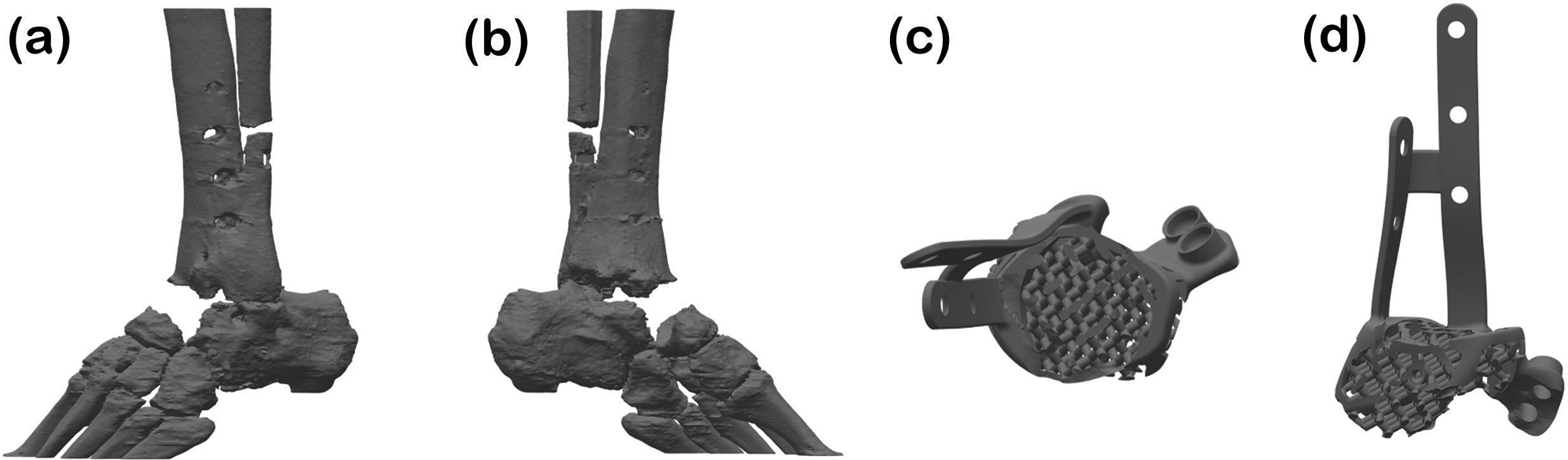
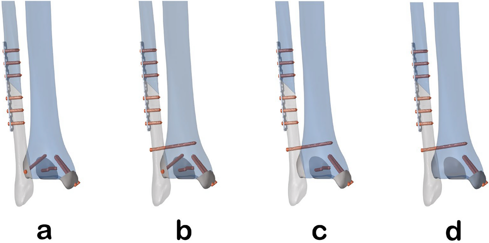
To reconstruct a three-dimensional model of a normal foot and ankle, we performed a foot and ankle scan of a 26-years-old healthy adult male volunteer (weight 60 kg, height 1.7 m, no history of foot trauma, tumors, or anatomical abnormalities on clinical examination). This study was conducted in accordance with the principles of the Declaration of Helsinki, and the volunteers provided written consent to participate in our study. The volunteer’s foot and ankle were kept in a neutral position during the CT scan (voltage of 120 kV, current intensity of 240 mA, scanning layer thickness of 0.600 mm). The CT data acquired from the scan were saved in DICOM format. The foot and ankle data were imported into Mimics21.0 (Materialise, Belgium) software in DICOM format, and 3D surface geometry reconstruction of the bones, including the tibia, fibula, and foot and ankle, was performed by threshold segmentation, region growing, and manual erasure. The STL files of the above bones were imported into the reverse engineering software Geomagic Wrap2021 (Geomagic Company, USA). Corrections were made in Geomagic Wrap for the presence of pegs, corners, and small holes, before fitting to the NURBS surfaces. The model was imported into SolidWorks2022 software (Dassault, France) in STP format, and the plate and screw models were established to simulate PER type IV ankle fracture, with the broken end of the fibula fracture 7 cm above the tibial dome, the area of the posterior ankle fracture accounting for 14% of the tibial talonavicular joint, the inner ankle fracture set to be a full cut angle of 30° horizontally, and the area of the anterior ankle fracture accounting for 5%. The parameters of the plate model were set to 88 mm in length, 8.5 mm in width, and 1.4 mm in thickness. There were three types of screws, lower tibiofibular joint fixation screw parameters were set to 3.4 mm in diameter and 52 mm in length, fracture fixation screw parameters were set to 3.4 mm in diameter and 37 mm in length, and the plate fixation screw technique was set to 3.4 mm in diameter and 10 mm in length. The models were sequentially assembled into four different internal fixation schemes, including a (all ankle fixation—utilizing a fibular plate and screws for comprehensive stabilization of the ankle), b (inferior tibiofibular joint fixation + all ankle fixation), c (inferior tibiofibular joint fixation + unfixed anterior ankle), and d (inferior tibiofibular joint fixation + unfixed anterior and posterior ankles) (Fig. 1). All models were imported into Hyperworks 2019 software (Altair, USA) in IGES format, frictionless face-to-face contact was used to represent the relative articular motion between layers of articular cartilage for frictionless sliding between the bones, and the ligaments were modeled using rod units that can only be stretched and not compressed based on anatomical information on the Digital Anatomy Platform and the Human Atlas. These ligaments were manually positioned and added to the model based on relevant anatomical landmarks.

Model of four different internal fixation modalities for the treatment of PER type IV ankle fractures. a All ankle fixation. b Inferior tibiofibular joint fixation + all ankle fixation. c Inferior tibiofibular joint fixation + unfixed anterior ankle. d Inferior tibiofibular joint fixation + unfixed anterior and posterior ankles

In this study, we used HyperMesh software to mesh the bones, cartilage, and soft tissues using tetrahedral grid cells with mesh sizes of 1 mm for cortical bone, 1 mm for cancellous bone, and 2 mm for peripheral soft tissues. Convergence tests were performed on the discretization of the finite element model until the calculated stress deviation was less than 5% (see Fig. 2), and the final model consisted of 509245 nodes and 2834755 elements. All bones, cartilages, ligaments, and base plates were assumed to be linearly elastic materials with continuity, full elasticity, homogeneity, and isotropy, and the base plate material was modeled as a rigid horizontal plate with a large Young’s modulus to simulate the ground. The material properties were obtained from the literature [15,16,17] (Table 1 lists the material properties of each element).

Convergence test results in terms of the von Mises stress

The coefficient of friction of the plantar contact with the rigid ground was set to 0.6. The subject weighed 60 kg, and in the standing phase, the right foot carried half of the body weight (300 N), and a load of 300 N was applied vertically upward through the rigid ground to simulate the plantar reaction force in balanced standing, with the tibia, fibula, and the upper surface of the soft tissues completely fixed in the constraints. In balanced stance, the Achilles tendon force is approximately 50% of the force applied to the foot [18], so a further vertical upward force of 150 N was applied to the Achilles tendon (Fig. 3a).

Overall model of the foot and ankle. a Applying boundary conditions and loading to the models. b Validation of model validity by plantar stress distribution

The boundary settings, load settings, and size of the finite element model vary from study to study, and in comparison with the model, the focus is on the comparison of stress distribution trends. The plantar stress distribution in this experimental model is in high agreement with the trend and magnitude of the plantar stress distribution in the finite element study by Tao [15] (Fig. 3b); thus, the foot and ankle model can be considered valid. The model can be used for finite element analysis and biomechanical studies of the foot and ankle joints.