
記住我


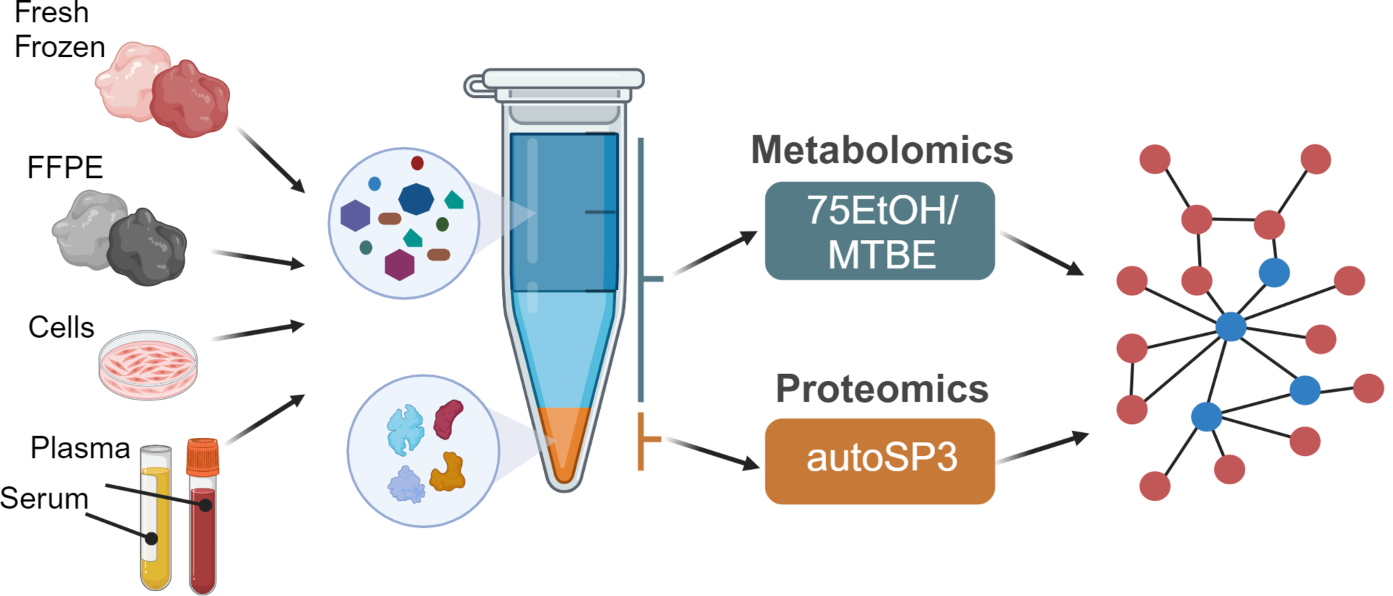
Here, we aimed to establish a strategy that combines two methods that had been individually optimised for proteome and metabolome analysis, i.e. SP3 and EtOH/MTBE, respectively, for integrated proteo-metabolomic analysis of physically the same sample. In particular, we used an organic solvents-based extraction to release metabolites, leaving a protein-containing pellet that we used as input material for SP3. In more detail, we applied a bi-phasic extraction with MTBE and 75% ethanol (EtOH) that precipitates proteins as a pellet and generates an upper organic phase containing lipids, and a lower aqueous phase containing polar metabolites (Fig. 1A). The liquid extract, containing the upper and lower phase (Fig. 1A), was transferred to a new reaction tube, dried, and resuspended for downstream targeted metabolomics via the Biocrates MxP Quant 500 kit while the pellet, containing the precipitated proteins (Fig. 1A), was used as direct input for the standard autoSP3 workflow, followed by a DDA approach on a timsTOF Pro mass spectrometer for proteome analysis [6, 9].
Fig. 1
Overview of experimental setup. (A) Proteins were extracted using two different methods: the established autoSP3 method and the single-sample workflow via 75EtOH/MTBE extraction followed by autoSP3 (MTBE-SP3). (B) The two extraction methods were tested and compared for several biological matrices (FFPE tissue, fresh-frozen tissue, cells, plasma, and serum). For FFPE and fresh-frozen tissue samples, tissue pieces (bulk) were either used as a direct input for autoSP3 or were cryo-pulverised and homogenised (powder). The powder was then used either as a direct input for autoSP3 (Powder-SP3) or subjected to the 75EtOH/MTBE extraction followed by autoSP3 (Powder MTBE-SP3). For serum, plasma and cells, samples were used either as direct input for autoSP3 or the biphasic 75EtOH/MTBE extraction followed by autoSP3 (MTBE-SP3). (C) To test the concordance between biological interpretations, both extraction methods were tested on a lung adenocarcinoma cohort and the resulting proteomes were compared
An important question is if proteome analysis of a sample that has undergone metabolite extraction and protein precipitation results in a bias in proteome composition or coverage, compared to the original autoSP3 approach that has been optimized for proteome analysis. This is relevant since autoSP3 extracts proteins using an SDS-containing buffer and does not include a protein precipitation step [9]. To test this, we performed comparative proteome analyses of samples prepared via MTBE-SP3 and autoSP3. This was evaluated for five different biological matrices: FFPE tissue, fresh-frozen tissue, plasma, serum, and cells (see methods for sample origin and further details on the biological matrices). Although FFPE tissue is not amenable for metabolome analysis, it was included here to assess potential bias of MTBE-based protein extraction in a wider diversity of samples. For each biological matrix we acquired three samples per extraction method (autoSP3, MTBE-SP3; Fig. 1) that were analysed for proteomics. For FFPE and fresh-frozen tissues, proteins were either extracted from bulk as a direct input to autoSP3 (Bulk-SP3) or from cryo-pulverised and homogenised tissue (Powder-SP3), or from the protein pellet obtained after 75EtOH/MTBE metabolite extraction (Powder-MTBE-SP3). Bulk FFPE and fresh-frozen samples were physically distinct tissue pieces, while samples from homogenised samples were taken from the same homogenate. For plasma, serum, and cell samples, proteins were extracted from the bulk (autoSP3) or from the pellet after 75EtOH/MTBE extraction (MTBE-SP3).
In a first analysis, we assessed the recovery of proteins based on the MaxQuant identification to check whether autoSP3 and MTBE-SP3 methods obtain similar sets of proteins (Supplementary Table S3). In terms of recovery of proteins in the two extraction methods, both protocols showed a high overlap of detected proteins (Fig. 2B, see also Fig. 2C for fresh-frozen tissue and Supplementary Figure S1 for data in other sample types). Looking at the shared protein identifiers after MaxQuant identification, the MTBE-SP3 method showed high overlap of detected proteins compared to the Powder-autoSP3/Bulk-autoSP3 in the FFPE (85%) and fresh-frozen samples (89.4%) and high overlap compared to autoSP3 in cells (97.6%), serum (90%) and plasma (91%). This indicates very similar efficiency of the extraction methods, which was also confirmed by the highly comparable LFQ intensity range in the respective proteomic datasets (Fig. 2A).
Fig. 2
Intensities and overlap across all sample types. (A) Densities of log-transformed LFQ intensities for the replicates in all sample types. (B) Bar chart illustrating the percentage of shared (common) and unique quantified proteins and peptides in MTBE-SP3 and autoSP3. (C) Joint and disjoint proteins and peptide sets in fresh-frozen samples. While some of the proteins and peptides were uniquely detected in one of the extraction methods (MTBE-SP3, autoSP3), the majority of proteins and peptides were detected in both methods. The numbers (in %) indicate the proportion of the largest set relative to the total number of proteins and peptides.(D) GRAVY and isoelectric point scores for proteins for the sets autoSP3/MTBE-SP3
Next, we evaluated whether MTBE-SP3 yields concordant proteomic results to the established autoSP3 protocol by the following measures: i) the number of differentially expressed proteins between the two extraction methods, ii) the correlation of log-transformed intensities of technical replicates, iii) and the precision of measurements expressed by the coefficient of variation (CV) of the technical replicates. i) We found a variable, but generally low number of proteins that differed in abundance (fresh-frozen tissue, powder: 0%; FFPE tissue, powder: 0%; cells: 1.1%; serum: 4.6%; plasma: 14.4%; FFPE tissue, bulk: 15.1%; fresh-frozen tissue, bulk: 19.3%). Especially the homogenised tissues showed no abundance differences between the two extraction methods, indicating their equivalent performance. In contrast, these numbers were higher for bulk samples, indicating that, as expected, non-homogenized samples exhibit higher variability in their protein content (Supplementary Table S1). ii) For FFPE and fresh-frozen samples, the correlation analysis between technical replicates revealed high CVs between MTBE-SP3 and (homogenised) auto-SP3 (average R2 = 0.80, SD = 0.05 for FFPE, and R2 = 0.91, SD = 0.02 for fresh frozen), and to a lesser extent between MTBE-SP3 and Bulk-SP3 (average R2 = 0.73, SD = 0.06 for FFPE and R2 = 0.82, SD = 0.04 for fresh frozen). For plasma, serum and cells high coefficients were obtained between MTBE-SP3 and auto-SP3 with an average R2 = 0.89, SD = 0.03 for plasma, R2 = 0.92, SD = 0.01 for serum, and R2 = 0.92, SD = 0.01 for cells. (Supplementary Figure S2). iii) Similar to autoSP3, MTBE-SP3 showed low CVs for liquid (plasma, serum), pulverised (fresh-frozen and FFPE tissue), and other matrices (cells, bulk fresh-frozen, and bulk FFPE tissue). While the differences in CV were significantly different between MTBE-SP3 and autoSP3 for most of the sample types (except serum, α < 0.05, no FDR correction), the effect size was generally low in absolute terms (Supplementary Table S1).
Moreover, we devised an R package (PhysicoChemicalPropertiesProtein, available via www.github.com/tnaake/PhysicoChemicalPropertiesProtein) to calculate two important parameters, the isoelectric point and GRAVY (grand average of hydropathy) scores, to scrutinise potential differences in extraction efficiencies regarding physico-chemical properties (Fig. 2D, Supplementary Figure S3). To that end, we correlated the values of the GRAVY/isoelectric point scores for proteins with the t-values from differential expression analysis. The t-values were regarded as a measure of how differently abundant proteins are for a given extraction method. The homogenous samples (FFPE (powder), cells, plasma, and serum), showed no clear association between the GRAVY/isoelectric point scores and t-values (Spearman ρ correlation coefficients close to 0). These small correlation coefficients were not statistically significantly different from 0, indicating that there is no bias in physico-chemical properties of proteins in the tissues FFPE (powder), cells, plasma, and serum. FFPE (bulk) and fresh-frozen tissue (powder and bulk) showed a moderate positive correlation between GRAVY scores and t-values (Supplementary Table S2). This suggests that more hydrophobic proteins were detected in higher abundance in these matrices in autoSP3 compared to the MTBE-SP3 extraction. Accordingly, GO terms related to the membrane system were differentially expressed between autoSP3 and MTBE-SP3 extraction in fresh-frozen tissue (bulk), while FFPE (bulk) showed enrichment of terms related to the cytoskeleton and DNA/RNA-related processes (Supplementary Figure S4). These differences may be explained from the fact that, by necessity, bulk samples were prepared from disparate tissue pieces which may have differed in composition. Therefore, in conclusion, our data show that depending on the tissue type MTBE-SP3 is equivalent to autoSP3 with regard to the proteome coverage that is obtained across a variety of sample types, with no noticeable (e.g. for fresh-frozen tissue, powder; FFPE tissue, powder; or cells) or moderate selectivity (e.g. FFPE tissue, bulk, fresh-frozen tissue, bulk) in protein extraction.
Applying MTBE-SP3 on a lung adenocarcinoma cohort yields similar results compared to autoSP3To demonstrate the advantages of the MTBE-SP3 workflow, we applied it in a combined proteome and metabolome analysis in a lung adenocarcinoma cohort. The cohort consisted of fresh-frozen samples from ten patients of paired tumorous tissue (TT) and non-tumorous adjacent tissue (NAT). A particular aim was to assess if similar biological conclusions can be reached in the comparison of these tissue regions when using autoSP3 or MTBE-SP3 for proteome analysis, despite minor differences that may exist between these methods. In addition, using MTBE-SP3, we performed broad-scale targeted metabolomics via MxP Quant 500 (Biocrates) (Supplementary Table S5). MatrixQCvis identified two low-quality samples, displaying a higher number of missing values and elevated median intensity levels compared to other samples, which were excluded from further analysis. In total, across all samples we quantified 6326 proteins in a single-shot DDA approach using a timsTOF Pro mass spectrometer (Supplementary Table S4). After filtering the data, proteomic data was available for 3010 protein features with quantitative information in > 50% of the samples, which were included for further analysis. The metabolomic dataset contained concentrations for 405 metabolites after applying the filtering steps based on the MetIDQ-derived quality scores (see Materials & Methods for further details).
To address if autoSP3 and MTBE-SP3 yield similar quantification results we determined if protein abundances differ when using them for protein extraction from either NAT or TT samples. Analysis of 10 vs. 10 NAT tissue pieces processed by autoSP3 and MTBE-SP3, respectively, identified 3010 proteins of which 809 showed a difference in abundance (α < 0.05 after FDR correction; 1113 significantly different features with α < 0.05 prior to FDR correction). For TT samples, 553 out of 3010 proteins showed an abundance difference (948 significantly different features with α < 0.05 prior to FDR correction). To test whether this difference may be explained by tissue heterogeneity, we run linear models for the two extraction methods separately on random, equally split partitions of samples. This analysis did not show any differentially expressed proteins for either autoSP3 or MTBE-SP3 (α < 0.05 after FDR correction, 130 and 235 significantly different features with α < 0.05 prior to FDR correction for MTBE-SP3 and autoSP3, respectively), indicating that tissue heterogeneity is not governing the observed differences. This suggests that slight differences exist between both methods for this type of samples, although fold changes were mostly modest. This is not necessarily problematic as long as no bias is introduced that skews biological differences between samples that are analysed with either method. To test this, we assessed if autoSP3 and MTBE-SP3 yield the same sets of differentially expressed proteins between NAT and TT samples. When looking at the NAT vs. TT differences adjusting for the autoSP3 and MTBE-SP3 methods (i.e., considering the differences between NATautoSP3vs. TTautoSP3 and NATMTBE−SP3vs. TTMTBE−SP3), only two proteins were significantly different (PDLIM2 and PRPF40A, α < 0.05 after FDR correction, Figs. 3A and 244 significantly different features with α < 0.05 prior to FDR correction), indicating the equivalence of both sample preparation methods.
Fig. 3
Differential expression analysis for lung adenocarcinoma cohort (proteomics). (A) UpSet plot of significant protein features for contrast autoSP3 vs. MTBE-SP3 (α < 0.05 after FDR correction). The DE analysis was performed on the sets corresponding to autoSP3 vs. MTBE-SP3 for NAT samples, autoSP3 vs. MTBE-SP3 for TT samples, and autoSP3 vs. MTBE-SP3 for the entire sample set. (B) UpSet plot for contrast TT vs. NAT. The DE analysis was performed on the sets derived from autoSP3 and MTBE-SP3 extraction. (C) Beeswarm plot of log fold changes. The sets correspond to the protein sets from panel B: ‘shared autoSP3’ corresponds to the log fold changes of the 1004 proteins in the autoSP3 dataset, ‘shared MTBE-SP3’ to the log fold changes of the 1004 proteins in the MTBE-SP3 dataset, ‘unique autoSP3’ corresponds to the log fold changes of the 382 proteins in the autoSP3 dataset, and ‘unique MTBE-SP3’ corresponds to the log fold changes of the 378 proteins in the MTBE-SP3 dataset. The absolute log fold changes in the shared sets are higher compared to the unique sets (autoSP3: W = 239,420, p-value < 4.2e-13; MTBE-SP3: W = 230,510, p-value < 3.6e-10; Wilcoxon rank sum test with continuity correction, no adjustment for multiple testing). (D) Scatter plot between t-values from MTBE-SP3 and t-values from autoSP3. The Spearman’s rank correlation ρ between the two sets of t-values is 0.83 (p-value < 2.2e-16, no FDR correction). DE: differential expression/differentially expressed. NAT: non-tumorous adjacent tissue. TT: tumorous tissue
We next determined the overlap among the proteins that were differentially expressed between NAT vs. TT, as obtained by autoSP3 and MBTE-SP3. The extraction methods detected 1386 (autoSP3) and 1382 proteins (MTBE-SP3) to be differentially expressed between NAT and TT (α < 0.05 after FDR correction; 1593 and 1568 significantly different features with α < 0.05 prior to FDR correction). Of these, 1004 proteins were shared among autoSP3 and MTBE-SP3, while 382 (autoSP3) and 378 (MTBE-SP3) were uniquely differentially expressed in each method (Fig. 3B). The considerably lower number of statistically differentially expressed proteins above (NAT vs. TT adjusting for the autoSP3 and MTBE-SP3 methods) compared to the high number of unique proteins for each method tested individually can be explained by the further introduction of variation and higher number of levels of fitted cofactors when adjusting for the two extraction methods. The magnitude of the fold-change among the 1004 shared proteins was higher compared to the 382 and 378 proteins that were unique to autoSP3 and MTBE-SP3, respectively (autoSP3: Wilcoxon’s W = 239,420, p-value < 4.2e-13; MTBE-SP3: Wilcoxon’s W = 230,510, p-value < 3.6e-10; Wilcoxon rank sum test with continuity correction, no adjustment for multiple testing, Fig. 3C), indicating that main differences were captured by both methods. The t-values of the contrast NAT vs. TT for autoSP3 and MTBE-SP3 showed a high correlation (Fig. 3D, ρ = 0.83, p-value < 2.2e-16, no FDR correction) indicating that both autoSP3 and MTBE-SP3 detected the same differential expression patterns between NAT vs. TT. Thus, although autoSP3 and MTBE-SP3 show slight differences in sampling proteomes from these tissues, they yield similar results when comparing differences between samples (here NAT vs. TT) adjusting for the extraction method. Taken together, the results indicate that autoSP3 and MTBE-SP3 perform similarly in quantifying proteome differences in complex clinical tissues.
Integration of metabolomic and proteomic dataFor the ten patients of the lung adenocarcinoma cohort, we additionally acquired metabolomic information using the Biocrates MxP Quant 500 assay. After performing quality control, the dataset contained information on the levels of 405 metabolites in the NAT and TT samples. Subsequently, we analysed the metabolomics dataset in conjunction with the MTBE-SP3 proteomics dataset, acquired from physically the same aliquot of the samples, and the autoSP3 proteomics dataset, acquired from a different aliquot of the samples (Fig. 1C). To characterise the coherence of the proteomic and metabolomic data at the level of biological processes, we determined if MSigDB hallmark enrichment scores computed from proteomic and metabolomic data were correlated and checked if this correlation differed when proteomic data were obtained by MTBE-SP3 or autoSP3. This showed notably that the hallmark scores were highly correlated (0.83 to 0.94 Pearson’s R) when considering only proteins, and that the inclusion of metabolites did not affect the hallmark scores much (Fig. 4A). Indeed, the number of measured metabolite features that could be mapped to metabolic pathways was not large enough to affect the correlation based on proteins. Nonetheless, we compared the hallmark scores that could be obtained specifically from proteomic or metabolic data, showing an average Pearson correlation of only 0.2 and 0.15 for MTBE-SP3 and autoSP3 proteomic data, respectively (Fig. 4B). This low correlation is consistent with the notion that metabolic abundance usually correlates poorly with the abundance of metabolic enzymes, even in the same pathways, further supporting that metabolomic data allows to generate complementary insights in combination with proteomic data. Furthermore, we observed no significant difference between the correlation coefficients of the MTBE-SP3 and the autoSP3 datasets (Fig. 4B, Student t-test p-value = 0.53, df = 3), indicating that both datasets are similar.
We then looked for more specific connections between enzymes and the overall metabolic deregulation profiles of tumours, and we assessed if they differ between MTBE-SP3 and autoSP3 datasets. The ocEAn package allows to explore connections between metabolites and metabolic enzymes beyond their direct interactions: ocEAn provides weighted interactions for all possible metabolites and enzymes of a reduced functional genome-scale metabolic network, where weights represent relative distances between metabolites and enzymes in the reaction network [25]. ocEAn was used to systematically explore metabolites upstream and downstream of metabolic enzymes, in order to determine which of those showed the most imbalanced metabolic abundance signatures between TT and NAT samples, i.e. enzymes that show very different metabolic abundance profile changes upstream and downstream of their respective reactions (Fig. 4C). Such imbalance can help to pinpoint metabolic bottlenecks in the metabolic reaction network, which can be more easily interpreted functionally than single metabolite abundance changes can. This notably showed that the succinate dehydrogenase (SDH) metabolic enzyme complex (composed of SDHA, SDHB, SDHC and SDHD), which converts succinate to fumarate as part of the Krebs cycle, was the most significantly imbalanced metabolic reaction according to metabolic deregulation in TT samples (Fig. 4D and E). Indeed, Fig. 4E shows that the abundance of proline and succinate, which are consumed upstream of the SDH complex, are also significantly down-regulated (thus located in the lower left quadrant), while the abundance of spermine, propionylcarnitine and acetylcarnitine, which are produced downstream of the SDH complex, is significantly increased (thus located in the upper right quadrant). Interestingly, the MTBE-SP3 and autoSP3 datasets showed a significant up-regulation of the SDHA complex subunit in TT, albeit more significant in the MTBE-SP3 dataset (MTBE-SP3: t-value = 3.80, p-value = 0.001 after FDR correction; autoSP3: t-value = 2.31, p-value = 0.04 after FDR correction). The marginal accumulation of carnitine conjugates, such as propionyl-carnitine and acetyl-carnitine (p-value = 0.06 and 0.27 respectively, after FDR correction, Fig. 4E) in TT, as well as the up-regulation of the SDH complex, can indicate a strong mitochondrial dysfunction, which is well captured by both proteomic datasets in combination with the metabolomic data. Furthermore, both MTBE-SP3 and autoSP3 datasets agreed on a significant down-regulation of the abundance of OGDH in TT compared to NAT (MTBE-SP3: t-value = 4.06, p-value = 0.005, after FDR correction; autoSP3: t-value = 5.7, p-value < 0.0001, after FDR correction), an enzyme of the TCA cycle converting α-keto-glutarate to succinyl-CoA, upstream of the SDHA complex in the TCA cycle (Fig. 4C), confirming a mitochondrial dysfunction. The integrated analysis of the proteomics and metabolomics datasets by ocEAn gives an additional perspective that is not directly recapitulated by a GO analysis of the proteomics dataset: The GO analysis mainly resulted in enriched terms related to RNA processing, gene expression, and translation (Supplementary Fig. 5). In the GO analysis of the autoSP3 dataset, seven terms in the category ‘Biological Process’ were related to mitochondrial processes linked to mitochondrial gene expression or translation, but no terms were linked to mitochondrial metabolism. For the ocEAn results, both datasets also agreed on the up-regulation of the PKM enzyme in TT, which is the final rate-limiting step of glycolysis (MTBE-SP3: t-value = 5.76, p-value < 0.0001, after FDR correction; autoSP3: t-value = 4.63, p-value < 0.0001, after FDR correction). Finally, the ocEAn scores estimated from the metabolomic data showed slightly higher correlation coefficients with the proteomic data of the MTBE-SP3 dataset than the autoSP3 dataset (MTBE-SP3/ocEAn Pearson correlation: r = 0.45, p-value = 0.05; autoSP3/ocEAn Pearson correlation: r = 0.36, p-value = 0.12). Thus, despite some sparse differences between autoSP3 and MTBE-SP3, the two methods performed equally well, leading to the same biological insight in an integrated proteomic and metabolomic analysis of clinical samples (Fig. 4A).
Fig. 4
Comparison of proteomic and metabolomic integration between MTBE-SP3 and autoSP3. (A) Pearson correlation coefficients between MTBE-SP3 and autoSP3 (i) proteomic MSigDB hallmark enrichment scores, (ii) integrated proteomic + metabolomic MSigDB hallmark enrichment scores, and (iii) averaged proteomic and metabolomic MSigDB hallmark enrichment scores. Hallmark enrichment scores were calculated using the decoupler package and represent the number of standard deviations away from the mean of an empirical null distribution of scores for a given hallmark. The colour gradient represents the correlation coefficient. (B) Pearson correlation coefficients between MTBE-SP3 proteomic and metabolomic MSigDB hallmark enrichment scores (left column), and Pearson correlation coefficients between autoSP3 proteomic and metabolomic MSigDB hallmark enrichment scores (right column). Hallmark enrichment scores were calculated using the decoupler package and represent the number of standard deviations away from the mean of an empirical null distribution of scores for a given hallmark. (C) Representation of the TCA cycle main enzymes and metabolites in ocEAn. Arrows represent consumptions (reactant to enzyme) and productions (enzymes to product) of metabolites. Colours represent positive (red, over-production and consumption) and negative (blue, under-production and consumption) metabolic ocEAn signature imbalance (signatures are defined as the sets of metabolites that are found upstream and downstream of a given enzyme in the whole metabolic reaction network). (D) Heatmap displaying the t-values of TCA enzyme abundance changes between lung TT and NAT for the autoSP3 and MTBE-SP3 dataset, and ocEAn metabolic imbalance scores estimated from the differential metabolomic abundances between lung tumour and healthy tissue. (E) Scatter plots representing the differential metabolomic abundances upstream (consumption) and downstream (production) of the SDH enzyme complex. The x-axis represents the ocEAn score, while the y-axis represents the corresponding t-value for a given enzyme (TT vs. NAT)
留言 (0)