Utility notation

Suppose that we are interested in risk assessment for some predetermined set of diseases, indexed \(i=1,...,I\), and are considering the genes \(j=1,...,J\) to be included in a panel for germline testing. We define an aggregate utility expression in terms of the following notation:

\(_=\\}\) is the indicator for developing disease i.

\(_=\\}\) is the indicator for testing positive for carrying a deleterious variant on gene j.

\(__=1,_=1} > 0\) is the utility associated with the scenario where the individual tests positive for carrying a deleterious variant on gene j and does develop disease i (abbreviated G + D+).

\(__=0,_=0} > 0\) is the utility associated with the scenario where the individual tests negative for carrying a deleterious variant for gene j and does not develop disease i (abbreviated G−D−).

\(__=0,_=1} > 0\) is the utility associated with the scenario where the individual tests positive for carrying a deleterious variant on gene j but does not develop disease i (abbreviated G + D−). Assume that \(__=0,_=1}__=0,_=0}\).

\(__=1,_=0} > 0\) is the utility associated with the scenario where the individual tests negative for carrying a deleterious variant for gene j but develops disease i (abbreviated G−D+). Assume that \(__=1,_=0}__=1,_=1}\).

We emphasize that the scenarios outlined by these definitions capture incomplete penetrance, as opposed to genotyping errors or misclassifying deleterious variants (DVs). In our notation, developing a disease (D+) refers to lifetime development of specific phenotypic features of a condition, and the converse (D−) refers to not developing those features. Let \(__=0,_=1}=__=0,_=0}-__=0,_=1}\) be the disutility associated with testing positive for gene j but not developing disease i (G + D−) or alternatively the utility benefit of testing negative for gene j and not developing disease i (G−D−), e.g., the disutility associated with unnecessary surveillance and over-treatment and possible anxiety due to a positive test. Similarly, define \(__=1,_=0}=__=1,_=1}-__=1,_=0}\) as the disutility associated with testing negative for gene j but developing disease i (G−D+) or alternatively the utility benefit of testing positive for gene j and developing disease i (G + D+), e.g., the disutility associated with default screening or preventive interventions relative to more intensive interventions along with false reassurance among those who go on to develop disease. We assume both \(__=0,_=1}\) and \(__=1,_=0}\) are greater than 0. In other words, we assume that if one does not develop the disease, testing negative for the associated DV leads to more beneficial outcomes, and if one does develop the disease, testing positive leads to more beneficial outcomes. (We do not consider situations where either \(__=1,_=0} < 0\) or \(__=0,_=1} < 0\), although we note that these may exist; for example, where the G−D+ utility is larger than the G + D+ utility and “the cure is worse than the disease”.) Finally, let \(__,_}\) be the disutility (potentially including psychological or physical harms) associated with conducting the test for gene j in relation to disease i, independent of test results. Then, the net utility for disease i in the setting where we test for gene j is

$$\begin &__=1,_=1}\Pr (_=1,_=1)+__=0,_=1}\Pr (_=0,_=1)+__=1,_=0}\Pr (_=1,_=0)+__=0,_=0}\Pr (_=0,_=0)+__,_}\\ = &\Pr (_=0)\left[\right.(__=0,_=0}-__=0,_=1})\Pr (_=1}_=0)+__=0,_=0}\Pr (_=0}_=0)\left.\right]\Pr (_=1)\left[\right.__=1,_=1}\Pr (_=1}_=1)+(__=1,_=1}-__=1,_=0})\Pr (_=0}_=1)\left.\right]+__,_}\end$$

(1)

Assuming that the utility associated with developing disease i in the absence of testing information for gene j is equal to \(__=1,_=0}\), and assuming that the utility for not developing disease i in the absence of testing is equal to \(__=0,_=0}\), then the net utility for disease i in the scenario where we do not test for gene j is

$$\begin&__=1,_=0}\Pr (_=1)+__=0,_=0}\Pr (_=0)\\=&(__=1,_=1}-__=1,_=0})\Pr (_=1)+__=0,_=0}\Pr (_=0)\end$$

(2)

Of interest is the difference in utility for disease i when testing vs. not testing for gene j, which we define as the difference between Eq. (1) and Eq. (2):

$$\begin___}=\Pr (_=0)[-__=0,_=1}\Pr (_=1}_=0)]+\Pr (_=1)[__=1,_=0}\Pr (_=1}_=1)]+__,_}\end$$

(3)

This difference in utility can be re-expressed in terms of \(\Pr (_=1)\), which is the prevalence for DVs of gene j, and \(\Pr (_=1|_=1)\), which is the cumulative lifetime risk or penetrance of developing disease i given that one is carries a DV in gene j (i.e., the penetrance):

$$\begin___}&=[__=0,_=1}\Pr (_=1)\Pr (_=0_=1)]+[__=1,_=0}\Pr (_=1)\Pr (_=1_=1)]+__,_}\\&=[-__=0,_=1}\Pr (_=1)(1-\Pr (_=1}_=1))]+[__=1,_=0}\Pr (_=1)\Pr (_=1}_=1)]+__,_}\\&=\Pr (_=1)\left[\right.__=0,_=1}+\left(__=0,_=1}\right.+__=1,_=0}\left.\right)\Pr (_=1_=1)\left.\right]+__,_}\end$$

(4)

It is beneficial to test for gene j when \(___} > 0\), which occurs when the utility for testing is greater than the utility for not testing. For simplicity, we will generally treat testing for a given gene as testing for a particular deleterious variant in the gene, but the framework readily extends to handle variant-specific tests, prevalences, and penetrances.

For multiple diseases (indexed by i) and tests (indexed by j), the aggregate utility Δ sums over all combinations of i and j. Doing so requires carrier prevalence and disease penetrance estimates for each gene and disease, as well as the specification of disutilities for testing positive for gene j but not developing disease i (G + D−), testing negative for gene j but developing disease i (G−D + ), and testing itself. Δ provides a simple summary value while still allowing genes to be evaluated individually:

$$\begin} &=\sum____}\\&=\sum_\left\_=0)[-__=0,_=1}\Pr (_=1_=0)]\right.\\&\qquad\left.+\,\Pr (_=1)[__=1,_=0}\Pr (_=1_=1)]+__,_}\right\}\\\quad&=\,\sum_\left\_=1)\left[-__=0,_=1}+\left(__=0,_=1}\right.\right.\left.\left.+\,__=1,_=0}\right)\Pr (_=1_=1)\right]+__,_}\right\}.\end$$

(5)

An additional \(__,_}\) can be included for each (i, j) combination (with perhaps less weight given for each additional test), or a single overall disutility for all testing can be used. Since Δ is the sum of the net utilities of particular disease-gene pairs (i, j), the decision as to whether or not to include a given test on a multi-gene, multi-disease panel depends only on the individual net utility of that test.

The number of disutility parameters \(__=0,_=1}\), \(__=1,_=0}\), and \(__,_}\) grows as the number of diseases and tests increases, but one can consider simplifications such as assuming the same (dis)utilities across diseases/tests or subgroups of diseases/tests. For example, it may be reasonable to assume that the disutility of each test for an additional gene j is negligible. Specification of these disutilities is largely subjective and should depend on the clinical setting and patient concerns.

Utility threshold

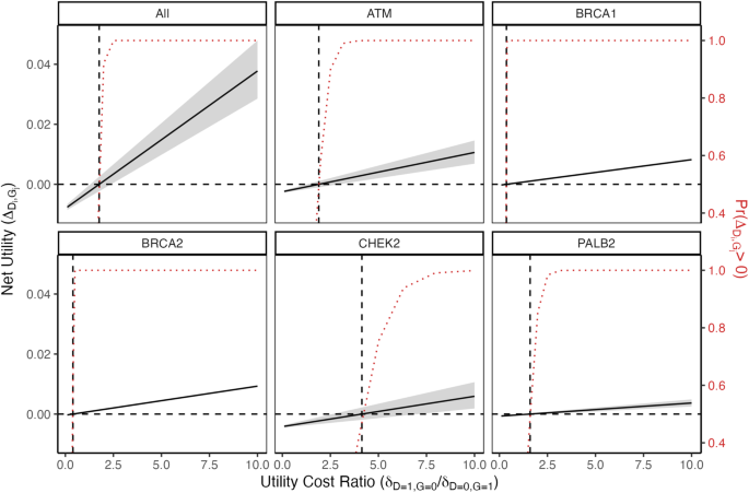
As a general guide for interpretation, if the user fixes the value of \(__=0,_=1}\), they can conceive of the value of \(__=1,_=0}\) as being a relative weight for the disutility of G-D+ vs the disutility of G + D−. More formally, for an individual test for disease i and gene j, a utility threshold can be defined as the value \(__,_}=__=1,_=0}/__=0,_=1}\) for which \(__,_}=0\):

$$\begin0&=__,_}\\&=\Pr (_=1)\left[-__=0,_=1}+(__=0,_=1}+__=1,_=0})\right.\left.\Pr (_=1_=1)\right]+__,_},\end$$

which implies

$$\begin\Pr (_=1)-(__,_}/__=0,_=1})=(1+__,_})\Pr (_=1_=1)\Pr (_=1),\end$$

so

$$__,_}=[1-(__,_}/__=0,_=1})/\Pr (_=1)]/\Pr (_=1_=1)-1.$$

(6)

Note that when \(__,_}=0\), \(__,_}=1/\Pr (_=1|_=1)-1\) and depends only on the penetrance \(\Pr (_=1|_=1)\). If the ratio of the disutility of G−D+ to the disutility of G + D− is greater than \(__,_}\), then including gene j to test for disease i has positive net utility. If the ratio needed to achieve a non-negative utility is unreasonable—e.g., in many settings ascribing a higher disutility to testing positive for the gene but not developing the disease compared to the disutility of testing negative for the gene but developing the disease would be inappropriate—then the test should not be kept as part of the panel. Basing analysis around a threshold ratio allows for an alternative interpretation that does not require upfront specification of the disutilities \(__=0,_=1}\), \(__=1,_=0}\), and \(__,_}\).

If one assumes that \(__=0,_=1}=_\) and \(__=1,_=0}=_\) for all values of i and j, then

$$\begin\Delta &=\sum _\left\_=1)\left[-_+(_+_)\Pr \left(_\right.\right.\left.\left.=\,1_=1\right)\right]+__,_}\right\}\\&=-_\sum _\Pr (_=1)\\&\qquad+\,(_+_)\sum _\Pr (_=1)\Pr (_=1_=1)+\,\sum___,_}\\&=_\left[\right.-\sum _\Pr (_=1)+\,\sum_(__,_}/_)+\\&\qquad\,(1+_/_)\sum_\Pr (_=1)\Pr (_=1_=1)\left.\right]\end$$

and the threshold \(b=_/_\) when Δ = 0 can be expressed as

$$\beginb&=&\sum_[\Pr (_=1)-(__,_}/_)]/\sum_\Pr (_=1)\Pr (_=1_=1)\left.\right]-1\\ &=&\sum_\Pr (_=1)/\sum_\Pr (_=1)\Pr (_=1_=1)\left.\right]-1,\end$$

(7)

where the last line holds when \(__,_}=0\) for all i, j.

Uncertainty distribution for disease penetrance

Of additional interest is the incorporation of uncertainty in the penetrance estimates \(\Pr (_=1|_=1)\). Denoting \(__,_}=\Pr (_=1|_=1)\) for a given disease i and gene j, we model the uncertainty in the penetrance \(__,_}\) as a beta distribution Beta(\(__,_}\), \(__,_}\)). One can motivate the choice of the parameters \(__,_}\) and \(__,_}\) by conceiving of the penetrance’s uncertainty distribution as the posterior distribution from a trial of \(__,_}\) carriers of deleterious variant j. Then, set \(__,_}=__,_}__,_}\) to represent the expected number of cases of disease i in the trial and set \(__,_}=__,_}__,_})\) to represent the expected number of individuals who do not develop the disease. Through specification of the precision \(__,_}\), we can express our confidence level in the estimation of \(__,_}\), with larger values of \(__,_}\) corresponding to a greater degree of certainty about the estimate and smaller ones indicating less confidence.

The uncertainty from \(__,_}\) can then be propagated into a distribution and credible interval for the corresponding \(__,_}\) and the aggregate Δ (assuming independence of \(__,_}\) across all i, j), as well as additional summary values. We will assume that we are not concerned about incorporating uncertainty from estimating \(\Pr (_=1)\). The probability that the individual net utility \(__,_}\) is positive (i.e., adding the test for gene j makes an improvement) can be written as

$$\begin\Pr (__,_} > 0)&=\Pr\left\_=1)[-__=0,_=1}+(__=0,_=1}+__=1,_=0})__,_}]\right.\left.+\,__,_} > \,0\right\}\\&=\Pr \__,_} >\, [__=0,_=1}-__,_}/\Pr (_=1)]/[__=0,_=1}+__=1,_=0}]\}\\&=\,\Pr \__,_} > \,__=0,_=1}/[__=0,_=1}+__=1,_=0}]\},\end$$

(8)

where the last line holds if \(__,_}=0\). \(\Pr (\varDelta > 0)\) does not generally have a closed form but can be calculated empirically from the sampling distributions of the \(__,_}\) s. One can also derive a lower bound on the estimated \(__,_}\) s that accounts for uncertainty by plugging in the fifth percentiles of the \(__,_}\) s in the uncertainty distributions in place of \(\Pr (_=1|_=1)\) in Eq. (6). This fifth percentile represents a “near-worst case scenario” for the net utility in which the true disease penetrance is at the low end of its credible range.

Reporting summary

Further information on research design is available in the Nature Research Reporting Summary linked to this article.