DNA labeling genome-wide

Earlier studies have employed various labeling techniques to mark chromatin, such as the insertion of ectopic DNA sequence arrays into chromosomes alongside ectopic expression of bacterial proteins that bind to these arrays, thereby labeling them. Additionally, specific genomic sequences have been visualized using techniques based on TALE or CRISPR/Cas9 (Ma et al. 2016, 2019) or the inclusion of ectopic sites such as LacO or TALE sites (Robinett et al. 1996; Vazquez et al. 2001; Dimitrova et al. 2008; Mach et al. 2022), where the TAL effector protein or catalytically inactive Cas9 protein binds to and labels specific loci. These methodologies have facilitated the study of chromatin dynamics across different processes, circumventing technical and analytical challenges associated with larger, clustered chromatin labels. However, it is important to note that these ectopic manipulations may introduce artifacts that do not accurately represent the true nature of chromatin.

To address this concern, we adopted the scratch loading technique, which involves the introduction of labeled deoxyribonucleotides into cells to label DNA directly (Cells) (Schermelleh et al. 2001; Sadoni et al. 2004).

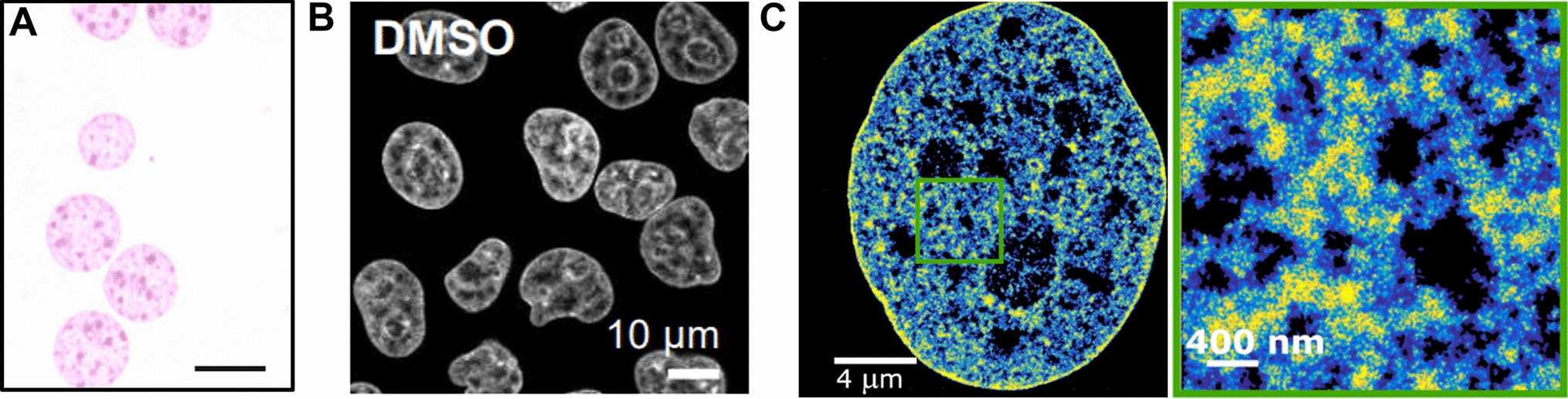
This method has proven effective for the rapid labeling of DNA in cells without altering their native chromatin state. The process of genome duplication, known as DNA replication, occurs during the synthesis (S) phase, where the chromosomes are duplicated. By directly labeling chromatin/DNA in replicating S phase cells, we can label any chromatin type (euchromatin, facultative heterochromatin, constitutive heterochromatin) as well as DNA repeat elements like LINEs and SINEs as well as tandem repeats, which are overlooked in most studies. As the human genome is GC poor, we selected dUTP for labeling. This is also advantageous over dCTP as the latter could interfere with cytosine modifications. Through the use of directly labeled deoxyribonucleotides and scratch loading, we can label the DNA genome-wide (Fig. 1A, B) and examine chromatin dynamics in its native state over several cell cycles. As a larger portion of genomic DNA is packaged into heterochromatin, this would be reflected also by this labeling method.

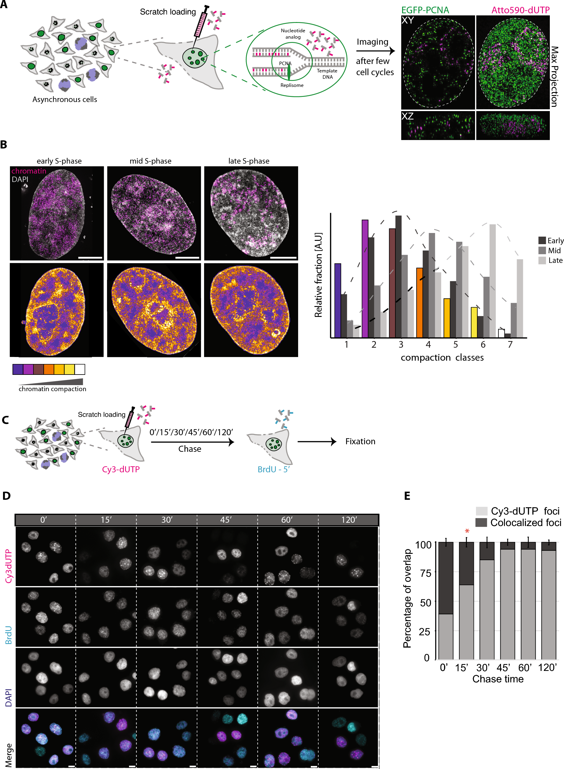
In our study, we utilized an asynchronous population of human HeLa K GFP-PCNA cells (Chagin et al. 2016; Pabba et al. 2023) containing fluorescently tagged proliferating cell nuclear antigen (PCNA). We labeled these cells using scratch loading with 100 µM ATTO590-dUTP (Methods, Supplementary Tables 1, 2). PCNA is a component of the DNA replication machinery and serves as a marker for cell cycle progression (Fig. 1A; Prelich et al. 1987; Leonhardt et al. 2000; Easwaran et al. 2005; Moldovan et al. 2007; Chagin et al. 2016; Pabba et al. 2023). The labeled cells were allowed to divide through multiple cell cycles, thereby distributing the label to daughter cells and increasing the population of cells with labeled chromatin. These labeled cells were then subjected to two-color 3D live-cell time-lapse correlative microscopy of an approximately 1-µm-high central subvolume acquired with 10-s intervals, where we obtained high-resolution 3D-SIM images along with the corresponding lower-resolution pseudo-WF images, generated from the same raw data. Additionally, we acquired multiple full Z stacks (volumetric imaging) per cell (Fig. 1A, Supplementary Fig. 1, Video 1, Microscopy). To cover cell populations in different cell cycle stages, we utilized GFP-PCNA patterns to select cells in specific stages for live cell microscopy. The representative images of a live mid S phase (GFP-PCNA focal pattern, green) cell with labeled chromatin (nucleotides, magenta) in pseudo-WF, deconvolved widefield (Deconv WF), 3D-SIM along with the zoom section are shown in Supplementary Fig. 1.

Given that the measurement of chromatin motion of labeled chromatin domains may depend on the size of the object (labeled DNA), it is imperative to assess the labeling duration and the size of the labeled DNA domains. This evaluation enables correlating between chromatin domain sizes and their diffusion rates. As the scratch loading method involves a short-term permeabilization and uptake of fluorescent dUTPs from the medium, the pulse duration cannot be controlled. Therefore, we conducted a pulse-chase-pulse experiment to determine the labeling/pulse duration. Briefly, we employed an asynchronous population of HeLa K GFP-PCNA cells and performed scratch loading with labeled nucleotides (1st pulse) to label replicating DNA (Methods, Supplementary Tables 1, 2). We then performed a chased of different durations (0′, 15′, 30′, 45′, 60′, 120′) and labeled the cells with a second pulse of 40 µM BrdU (5-bromo-2′-deoxyuridine, a cell-permeable nucleoside), followed by fixation and detection of BrdU using antibodies (Fig. 1B, C; Double pulse analysis to determine the labeling duration; Supplementary Tables 2, 3). We then performed high-throughput imaging, which allowed us to obtain a larger cell population for quantification (Fig. 1C, Supplementary Table 4). We segmented the nuclei marked by DAPI staining and DNA foci labeled with fluorescently labeled nucleotides (1st pulse, magenta, scratch loading) and BrdU (2nd pulse, cyan, nucleoside) channels and performed colocalization analysis between the pulses to calculate the percentage of labeled nucleotides foci overlapping with BrdU foci (Fig. 1C, Supplementary Fig. 2, Supplementary Tables 5, 6). The lack of colocalization is used as a proxy for the duration of the first pulse. Our findings indicate that the nucleotide pulse during scratch loading is primarily incorporated into the genome within the initial 15 min, providing insight into the labeling duration of DNA/chromatin (Fig. 1D).

Quantification of the size of labeled chromatin domains

As the chromatin diffusion/dynamic rates may be influenced by the chromatin domain sizes, we wanted to investigate the DNA domain sizes that were labeled within the 15 min of labeling duration after scratch loading. Hence, we performed microscopic imaging at different modes of resolution (WF, WF deconvolution, and super-resolution 3D-SIM) to quantify the corresponding labeled DNA domain sizes.

In previous studies, we have quantified the genome size (GS) of HeLa K cells to be GS = 9.682 ± 0.002 Gbp (Chagin et al. 2016). During S phase the genome is duplicated, whereby the total DNA is doubled from G1 to G2 progression before cell division in mitosis. Therefore, to precisely measure the relative DNA amount during S phase we utilized flow cytometry to determine the relative DNA amounts during the cell cycle progression (Supplementary Fig. 3). Briefly, we used ice-cold methanol-fixed HeLa K GFP-PCNA cells labeled with the DNA/RNA dye PI in combination with RNase A (to remove the RNA detection) and performed flow cytometry to detect the total amount of DNA. We then plotted the total DNA (PI) intensity on the x-axis and the number of cells on the y-axis (Methods, Supplementary Fig. 3). The DNA intensity profile over the cell cycle was fitted with the aneuploid profile of HeLa K cells (Metaphase spreads, Supplementary Fig. 4), to obtain the relative DNA amount present in early, mid, late S phase cell cycle stages. Using these data we obtained the cell cycle correction factor (C; G1—1, eS—1.06, mS—1.27, ls—1.71, G2—1.98) for all cell cycle stages (Supplementary Fig. 3).

To quantify the DNA domain sizes, we subjected HeLa K GFP-PCNA cells to scratch loading with Cy3-dUTP followed by chemical fixation using formaldehyde (DNA quantification of labeled chromatin, Supplementary Tables 1, 2). The total DNA was subsequently stained with DAPI. We performed fixed cell imaging of DAPI (total DNA), GFP-PCNA (green), and Cy3-dUTP (labeled chromatin) and imaged the whole nuclear volume in SIM and WF resolutions (voxel size 41 ×  41 ×  125 nm). Then, we segmented both the entire nucleus and the individual labeled chromatin foci within the same cell. The fraction of DAPI intensity within the segmented replication focus (IRFi) relative to the total DNA intensity within the cell (IDNA total) provided the amount of DNA per labeled chromatin focus (DNA quantification of labeled chromatin, Fig. 2A, Supplementary Fig. 5). The DNA content (kbp) present in each labeled foci for SIM and WF images (N = 30) was plotted as a histogram where the x-axis represents the DNA amount present per focus (kbp) and the y-axis represents the count (Fig. 2A). The mode and median values of the histogram are indicated in Fig. 2A. We observed that in WF microscopy, a large number of labeled foci with a DNA content ranging from 100 to 500 kbp of DNA (median 210 kbp), which correspond to TAD-like structures (Giorgetti and Heard 2016). Whereas, using super-resolution microscopy (SIM), a large number of labeled foci have a size between 100 and 200 kbp of DNA (median 110 kbp), which corresponds to smaller loop like structures as shown by previous studies (median 185 kbp) (Rao et al. 2014; Mamberti and Cardoso 2020). Therefore, we propose that replication labeled DNA domains resolved by conventional WF microscopy correspond to TAD-sized domains whereas DNA domains resolved by 3D-SIM correspond to chromatin loops or sub-TADs. This is solely based on DNA content but not DNA sequence and need not correspond to TADs and loops identified by Hi-C methods.

Fig. 2

Quantification and correlation of labeled replication domains using microscopy and single molecule DNA fibers. A HeLa K GFP-PCNA cells were labeled with Cy3-dUTP (magenta) (Supplementary Table 2) using scratch loading technique and were then fixed using 3.7% paraformaldehyde for 15 min and DNA was stained using DAPI. The cells were then imaged using the DeltaVision OMX microscope for both GFP-PCNA and Cy3-dUTP (Supplementary Tables 1, 2, 3, 4) and processed to display corresponding widefield and 3D-SIM images. GFP-PCNA patterns were used to determine the cell cycle stage and the cell cycle correction factor (Supplementary Figs. 3, 4). Representative images of DNA (DAPI—gray) and labeled chromatin (Cy3-dUTP—magenta) in WF and 3D-SIM resolution  are shown. Individual cells were segmented, analyzed, and corrected for genome size and the histograms representing the quantified DNA amount per focus (N = 30) was plotted. The mode ± 5 bin of the histogram was represented in the figure (DNA quantification of labeled chromatin, Supplementary Figs. 3, 4, 5). The statistics of the histogram are shown in Supplementary Table 6. Scale bar 5 µm. B Single molecule DNA fiber experiment of DIG-dUTP labeled cells was performed to estimate the labeling efficiency of cells and correlate the DNA domain quantification using microscopy (DNA combing, Supplementary Figs. 6, 7, Supplementary Tables 3, 4). C Representative image of a single linearly stretched DNA fiber (cyan) and the labeled replication foci (DIG-dUTP: magenta). D The DNA fiber length and the labeled replication foci in kbp were plotted using the calibration measurements performed using lambda DNA (Supplementary Fig. 7). Scale bar 100 kbp

To validate our results with an orthogonal method, we employed DNA fiber combing to quantify the labeled chromatin domain sizes using a single molecule DNA fiber method (Parra and Windle 1993; Bensimon et al. 1994; Jackson and Pombo 1998; Daigaku et al. 2010; Técher et al. 2013; Moore et al. 2022). This allowed us to visualize the labeled DNA domains and translate the 3D chromatin structures into linear DNA fibers (Fig. 2B). To get significant results, we needed to optimize the DNA combing technique to obtain long stretches of DNA fibers up to 4 Mbp (commonly the fibers break after a few hundreds of kbps) to be able to visualize multi-loop domains. Briefly, we labeled HeLa K cells with 100 µM DIG-11 dUTP nucleotides using electroporation to enable nucleotides to enter cells. The cells were then allowed to recover from electroporation overnight and DNA strands were extracted into the DNA combing buffer (DNA combing, Supplementary Fig. 6). Using antibodies we detected the incorporated DIG-11dUTP signal (magenta) on the linear single genomic DNA fibers (YOYO, cyan) (Fig. 2C). We performed the calibration of DNA stretching using the Genomic Vision combing machine to determine the stretching factor using lambda DNA (48.5 kbp) and obtained a stretching factor of 1 µm = 2 kbp (DNA combing, Supplementary Fig. 7). We then used the calibration results to measure and plot a histogram with the size of DNA fibers (cyan) in kbp and the size of labeled nucleotides in kbp (magenta) present along the DNA fibers (Fig. 2D). The DNA fiber results showed that the labeled DNA domains are between 50 and 100 kbp in size, which corresponds to our DNA content measurements using 3D-SIM imaging.

Correlative chromatin motion analysis shows that nano-foci chromatin loops are more mobile than larger TAD-like structures

To perform correlative chromatin motion analysis, we imaged live HeLa K GFP-PCNA cells labeled with ATTO-590dUTP using scratch loading and performed dual-channel, multi-resolution, 3D sub-volume time-lapse imaging (frame interval of 10 s, 7 z-sections, 12 frames), to analyze and compare chromatin motion at different resolutions (Fig. 3A, Cells, Microscopy). During the acquisition of time-lapse movies, we observed a significant movement and deformation of the cells. We overlaid the chromatin channel from time point 1 (T1, magenta) and the final time point (T12, cyan) and observed a unidirectional motion of chromatin foci, which corresponds to cell movement (Supplementary Fig. 8). As there are fewer labeled chromatin foci in the nuclear sub-volumes, identification of nuclear boundaries was not possible in the chromatin channel. Therefore, we utilized the PCNA channel to segment the nuclear outlines. To register the time-lapse movies, we performed affine registration using our previous deep learning method to correct for rotational and translational motion of cells (Celikay et al. 2022). To correct for deformations of the nucleus during time-lapse microscopy, we used non-rigid registration after affine registration (Balakrishnan et al. 2019) improving the tracking accuracy considerably (Registration of live-cell image data, Video 2). To ensure that the particle detection algorithm only detects true chromatin foci, but not high-frequency noise artifacts generated during the SIM reconstruction, we used fixed control cells to detect any small-scale structures and their motion (Supplementary Fig. 9-A). This allowed us to optimize the particle detection threshold to detect true chromatin foci and perform tracking reliably (Supplementary Fig. 9-A, Methods). We also checked the number of chromatin foci detected over time in SIM and WF time-lapse movies. We observed a threefold increase in the number of foci detected between higher and lower resolution imaging (Supplementary Fig. 9-B, C). Having these controls, we then performed correlative motion analysis to obtain MSD (µm2) over time intervals in seconds (s) (Supplementary Fig. 10). We plotted the MSD curves for SIM (green), WF (blue), and fixed cells (gray) over time intervals (Fig. 3B, Video 3). In the SIM resolution datasets, we measured a diffusion constant (D) of 8.32 × 10−5 µm2/s with an alpha value (α) of 0.95, whereas with WF resolution the diffusion constant was lower with a D of 5.44 × 10−5 µm2/s and an alpha value (α) of 0.76 (Fig. 3C). We found that the chromatin nano-foci structures or loops imaged at SIM resolution are considerably more mobile than the clustered TAD-like domains imaged at WF resolution (Fig. 3D, Videos 3, 4). We next measured the radius of gyration (µm), which describes the extent of motion (Rg) of a chromatin polymer over time and visualized it using box plots. We observed that chromatin foci in SIM (green) (mean 0.0818, median 0.0763) have a higher radius of gyration compared to chromatin foci in WF (blue) (mean 0.0738, median 0.0699) (p < 0.001) (Fig. 3E). We measured the mean particle size (in µm3), which allowed us to correlate the radius of gyration with the particle size and plotted these using box plots. We observed that chromatin foci in SIM (green) (mean 0.01267, median 0.008685) have significantly lower volumes compared to chromatin foci in WF (blue) (mean 0.02564, median 0.01121) (p < 0.001) (Fig. 3F). As a result of the higher chromatin domain sizes, we see a lower radius of gyration for chromatin foci in WF compared to SIM.

Fig. 3

Correlative chromatin mobility of labeled DNA in HeLa K cells at widefield and structured illumination microscopy resolution. A HeLa K cells expressing GFP-PCNA were labeled with ATTO-590-dUTP (Methods, Supplementary Tables 1, 2) using scratch loading. After a few cell cycles, live cells were imaged in 3D and processed for structured illumination microscopy (SIM) and widefield (WF) resolutions, and time-lapse movies (frame interval of 10 s) of both GFP-PCNA (green) and labeled chromatin (magenta) were obtained (Supplementary Table 4). Representative images of HeLa K cells with PCNA (green) and labeled chromatin (magenta) in SIM and WF are shown. Inserts (white—1, 2) represent the zoom of chromatin imaged with SIM and WF resolutions, respectively. The zoomed inserts also show the computed tracks of chromatin over time (Supplementary Fig. 8, Videos 1, 2, 3, 4). B Non-rigid registration of the time-lapse movies using PCNA-GFP was performed to correct for the movement of cells (Methods, Supplementary Fig. 9). The registered movies were then used to detect labeled chromatin foci (Methods, Supplementary Fig. 10). These chromatin foci from the time-lapse movies of both SIM and WF were then analyzed to obtain the mean squared displacement curves (MSD, µm2) over time intervals (s) (Supplementary Fig. 8). MSD curves (µm2) over time intervals (s) for SIM (green), WF (blue), and control fixed cells (gray) were then plotted. C The table details the values of the anomalous diffusion coefficient α and the diffusion coefficient D (µm2/s × 10−5). D Illustration of labeled chromatin and its chromatin motion in SIM and WF. E, F Radius of gyration (µm) and mean particle size (µm3) for SIM (green) and WF (blue) chromatin domains (Supplementary Fig. 11). There is a highly significant difference between the SIM and WF foci (p < 0.001). The median and mean of the measurements are indicated in the figure. G Mean velocity (µm/s) of labeled chromatin foci for SIM (green) and WF (blue) plotted as a curve over time (s). H Mean velocity (µm/s) of labeled chromatin foci for SIM (green) and WF (blue) plotted as a box plot. There is a highly significant difference between the SIM and WF foci (p < 0.001). The median and mean values of the measurements are indicated in the figure. The statistics of the plots are shown in the figure and listed in Supplementary Table 6. Scale bar 5 µm. Also see Videos 1, 2, 3, 4

We then asked the question whether the mean velocity (µm/s) of chromatin foci in SIM is higher than for WF. We plotted the velocity curves and box plots for SIM (green, mean 0.006042, median 0.005854) and WF (blue, mean 0.005895, median 0.005598, and p = 0.09825) and observed no significant difference between the mean velocities of chromatin at different resolutions (Fig. 3G, H). We also measured the track straightness and the start-to-end distance and observed a significant difference between SIM (green) and WF (blue) chromatin foci (p < 0.005) (Supplementary Fig. 11, Supplementary Table 6). In summary, our results characterize the chromatin motion differences in smaller loop chromatin domains and larger TAD-like domains, which helps us to relate chromatin dynamics in the context of chromatin higher-order organization.

Chromatin motion reduces in S phase relative to G1/G2

To determine how the global chromatin dynamics change during cell cycle progression at multiple resolutions (SIM and WF), we utilized chromatin labeled cells and GFP-PCNA to assign the cell cycle stage during S phase (Leonhardt et al. 2000; Sadoni et al. 2004; Chagin et al. 2016). First, the cells were annotated according to the different cell cycle stages (G1, S, G2) based on the PCNA subnuclear pattern (Methods). PCNA forms puncta or foci at the active replication sites during S phase, which was used to classify cells in S phase. We were able to distinguish between G1 and G2 cells, even though they exhibit a similar diffused PCNA subnuclear distribution, based on the information on the preceding cell cycle stage from the time-lapse analysis performed after labeling (Microscopy). Specifically, cells with diffusely distributed PCNA signal, which had previously undergone mitosis were in G1 phase, whereas the ones with similar diffuse PCNA pattern that had previously undergone S phase (punctated PCNA pattern) were classified as being in G2 phase. The PCNA signal was also used to segment the nucleus, and individual chromatin foci were detected within the segmented nuclei. Probabilistic tracking was performed to obtain individual chromatin trajectories at SIM and WF resolutions. Representative images of GFP-PCNA (green) and labeled DNA (magenta) of mid S phase and G1/G2 cells along with chromatin tracks are shown in Fig. 4A, Video 5. We performed probabilistic chromatin tracking (Supplementary Fig. 10, Methods) to obtain the MSD (µm2) over time intervals (s) of S phase versus non-S phase at different resolutions (Fig. 4B, Supplementary Fig. 12-A). The curves show significantly higher chromatin dynamics in SIM G1/G2 [light green, diffusion coefficient (D) = 13.01× 10−5 µm2/s] compared to SIM S phase [dark green, diffusion coefficient (D) = 7.05 × 10−5 µm2/s]. We also observe a significantly higher chromatin dynamics in WF G1/G2 (light blue, diffusion coefficient (D = 7.95 × 10−5 µm2/s) compared to WF S phase [dark blue, diffusion coefficient (D) = 4.95 × 10−5 µm2/s] (Fig. 4C, Supplementary Fig. 12-A). In summary, we see reduced chromatin motion in S phase compared to non-S phase independent of the resolution. These results concur with our previous observations at confocal resolution (Pabba et al. 2023). It is also interesting to see that the S phase chromatin mobility in SIM is lower than the G1/G2 chromatin mobility in WF, showing that there are more constraints in chromatin loop motion in S phase than the larger TAD-like domains.

Fig. 4

Correlative motion analysis of labeled chromatin during the cell cycle stages and depending on temperature. A HeLa K cells with labeled DNA were used to obtain live-cell time-lapse movies (frame interval of 10 s) (Methods, Supplementary Tables 1, 2). Correlative imaging of two channels GFP-PCNA and labeled chromatin in SIM and WF in 3D were obtained (Supplementary Table 4). During S phase, PCNA accumulates within the nucleus at sites of active DNA replication and exhibits a distinct puncta pattern. During G1 and G2, GFP-PCNA is diffusely distributed throughout the nucleus. GFP-PCNA patterns were used to classify cells in different cell cycle stages (Supplementary Fig. 3). The representative images show GFP-PCNA (green) and labeled DNA (magenta) for both SIM and WF resolutions. The tracks of chromatin mobility of the white inserts are shown in zoom. B The registered time-lapse movies were used to detect chromatin foci of both SIM and WF and then analyzed to obtain the mean squared displacement curves (MSD, µm2) over time intervals (s) (Supplementary Figs. 8, 13). The MSD curves over time intervals (s) were plotted for S phase and G1/G2 for both SIM and WF. C The table details the values of the anomalous diffusion coefficient α and the diffusion coefficient D (µm2/s × 10−5). D Illustration of labeled chromatin and in S phase and G1/G2. E During live cell imaging of chromatin labeled HeLa K GFP-PCNA cells, experiments at two different temperatures (37 ºC and room temperature (RT)) were performed. The MSD curves over time intervals (s) were plotted for imaging at 37 °C and RT for both SIM and WF (Supplementary Fig. 12). F The table details the values of the anomalous diffusion coefficient α and the diffusion coefficient D (µm2/s × 10−5). The statistics of the plots are shown in figure and listed in (Supplementary Table 6). Scale bar 5 µm. See Video 5

Chromatin motion reduces with decreasing temperature at different resolutions

To analyze the changes in chromatin mobility at different temperatures, we acquired 3D live-cell time-lapse images (frame interval of 10 s) of HeLa K GFP-PCNA, and labeled chromatin (ATTO590-dUTP) at 37 °C and RT (Microscopy, Supplementary Tables 1, 2, 4) and plotted the MSD curves for both conditions 37 °C and RT at different resolutions (Fig. 4E, Supplementary Fig. 12-B). The MSD curves show significantly higher chromatin dynamics in SIM at 37 °C [dark green, diffusion coefficient (D) = 8.32 × 10−5 µm2/s] compared to SIM at RT [light green, diffusion coefficient (D) = 3.97 × 10−5 µm2/s]. We also observe that the results show significantly higher chromatin dynamics in WF at 37 °C (dark blue, diffusion coefficient (D) = 5.44 × 10−5 µm2/s) compared to WF at RT [light blue, diffusion coefficient (D) = 2.73 × 10−5 µm2/s] (Fig. 4E, F; Supplementary Fig. 12-B). We found that regardless of the resolution, the chromatin mobility at 37 °C is significantly higher than at RT.

Motion subpopulation analysis of chromatin shows different diffusion behaviors

We next asked the question whether chromatin foci at SIM resolution (loops) or WF resolutions (“TADs”) behave differently in terms of chromatin motion. To answer this, we classified the chromatin foci tracks into two distinct motion populations (0—red, 1—yellow) using k-means clustering of the anomalous diffusion coefficient α at both SIM and WF resolutions (Fig. 5A). The subpopulation mean values of α for SIM are 0.56 and 1.66 for population 0 (red) and population 1 (yellow), respectively, and the subpopulation mean values of α for WF are 0.48 and 1.63 for population 0 (red) and population 1 (yellow), respectively (Supplementary Table 6). For these subpopulations, we computed and plotted the MSD (µm2) over time intervals (s) for SIM and WF microscopy (Fig. 5B). We observed that chromatin foci of population 0 (red) exhibit a constrained diffusion behavior at both SIM (mean α = 0.56) and WF (mean α = 0.48) resolutions as suggested by various studies (Marshall et al. 1997; Heun et al. 2001; Chuang and Belmont 2007; Oliveira et al. 2021; Pabba et al. 2023). To our surprise, we also observed a minor population of chromatin foci or population 1 (yellow) showing directed diffusion behavior at both SIM (mean α = 1.66) and WF (mean α = 1.63) resolutions (Fig. 5B, Supplementary Table 6). This effect was predominant in higher-resolution chromatin loops domains than compared to lower-resolution TADs (Fig. 5B).

Fig. 5

Subpopulation classification of chromatin motion. A Representative images of HeLa K GFP-PCNA (green) and labeled chromatin (magenta) live cells in SIM and WF. The computed chromatin tracks were classified into population 0 (red) and population 1 (yellow) based on k-means clustering of the α values. The tracks were colored in red (population 0) and yellow (population 1) in both SIM and WF images. The subpopulation mean values of α for SIM are 0.56 and 1.66 for population 0 (red) and population 1 (yellow), respectively. The subpopulation mean values of α for WF are 0.48 and 1.63 for population 0 (red) and population 1 (yellow), respectively. We analyzed different parameters for different subpopulations and plotted them (Supplementary Fig. 13). B Mean squared displacement (MSD, µm2) over time intervals (s) for population 0 (red) and population 1 (yellow) was plotted for SIM and WF time-lapse movies. We also plotted the mean distance (µm) to the cell border for the chromatin tracks of the subpopulations. There is no significant difference in mean distance (µm) to the cell border between the subpopulations. The mean and median of the box plots are also indicated. The statistics of the plots are shown in figure and listed in (Supplementary Table 6). C The mean particle size (µm3) of SIM and WF chromatin domains of population 0 (red) and population 1 (yellow) are plotted as box plots. There is no significant difference between the populations. The mean and median of the box plots are also indicated. D The track straightness of SIM and WF chromatin domains of population 0 (red) and population 1 (yellow) are plotted as box plots. There is a highly significant difference between the two populations (p < 0.001). The mean and median of the box plots are also indicated. E The distance start–end (µm) of SIM and WF chromatin domains of population 0 (red) and population 1 (yellow) are plotted as box plots. There is a highly significant difference between the two populations (p < 0.001). The mean and median of the box plots are also indicated. The statistics of the plots are shown in figure and listed in (Supplementary Table 6). Scale bar 5 µm

We then asked the question whether there is a relation between the two motion populations and their spatial location. To answer this, we plotted and visualized the mean distance (µm) of each chromatin foci from the cell border of population 0 (red) and population 1 (yellow) at both resolutions. We observed no significant difference between the two populations in SIM and WF resolution (Fig. 5B). We then measured and visualized different parameters such as mean particle size (µm3), track straightness, and distance start–end (µm) for SIM and WF (population 0 and population 1). We observed no significant difference in particle size (µm3) between population 0 and population 1 for both SIM and WF chromatin foci (Fig. 5C, Supplementary Fig. 13, Supplementary Table 6). It is interesting to observe