
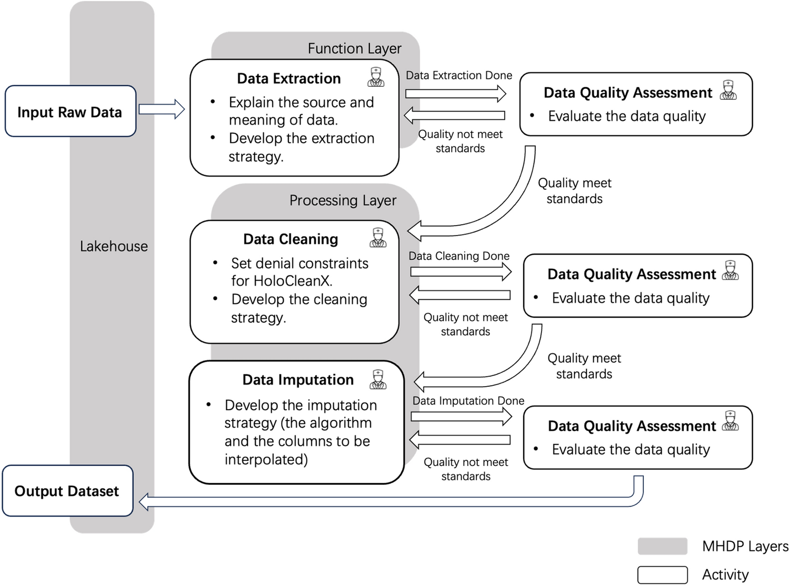
記住我
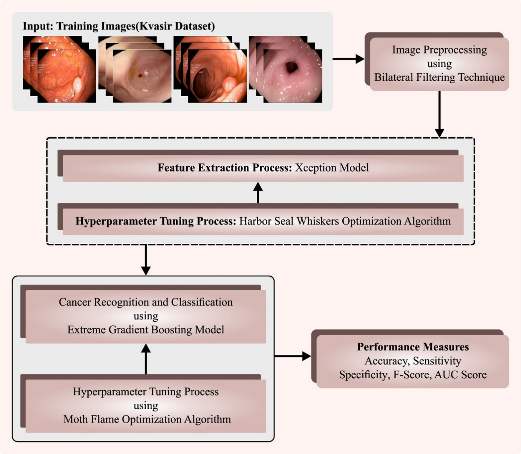


Numerous experimental analyses have been conducted to thoroughly examine the performance of the SAC model. These empirical investigations are presented in this section. Following this, the section elaborates on hyperparameter settings. Subsequently, the SAC model is contrasted with studies in the Kvasir dataset literature and state-of-the-art models like ViT, Swin Transformer, ConvMixer, and MLPMixer. Finally, the SAC model behavior analysis was performed for the Kvasir dataset using GradCAM (Gradient-weighted Class Activation Mapping).
Settings of hyperparametersWe utilize a specific arrangement of hyperparameters to train our SAC architecture using the TensorFlow library within the Google Colab, which includes a Tesla T4 GPU and 2× Intel(R) Xeon(R) CPU @ 2.30 GHz paired with 12GB of RAM, offering ample computational capability for our training requirements. Overall, we anticipate that the conjunction of hyperparameters, callbacks and optimizers with TensorFlow in the Google Colab setting will facilitate achieving cutting-edge outcomes with our SAC architecture. Our hyperparameters encompass validation split, image size, batch size, learning rate (lr), weight decay, number of epochs, filters, depth, kernel size, and patch size. Specifically, the proposed SAC model is divided into 70% training, 15% testing, and 15% validation dataset. The images were trained with an image size of \(128 \times128\) pixels and a batch size of 32. Additionally, we set the learning rate (lr) to 0.001, the weight decay to 0.0001, and performed training for 25 epochs. The architecture incorporates 256 filters, a depth of 8 with a patch size of 2 and a kernel size of 5. Additionally, To optimize the architecture and minimize the loss function, we utilize the AdamW [44] optimizer. Aside from the hyperparameters, we incorporate two distinct callbacks to enhance the training procedure. The initial callback, ReduceLROnPlateau, functions to diminish the lr when the validation loss plateaus, preventing overfitting and ensuring stability in training. The subsequent callback, ModelCheckpoint, saves the model weights periodically throughout training, enabling us to preserve the best model according to validation accuracy, ensuring its availability for subsequent use.
The proposed SAC model was evaluated on the Kvasir dataset. The assessment of the SAC model’s efficiency relied on evaluation metrics like F1-score (F1s), precision (Pr), recall (Re) and accuracy (Acc). These metrics offer an objective quantitative measure, crucial in appraising a architecture’s predictive efficacy and identifying potential enhancement areas. Each criterion offers a specific viewpoint on the architecture’s performance, each with its particular strengths and drawbacks. Below, a comprehensive elucidation of these metrics is provided.
The metric of Acc (Eq. 1) serves as a fundamental evaluation measure, determining the proportion of correct predictions derived from the architecture. It is computed by dividing the count of accurate predictions by the overall number of predictions. Nonetheless, when dealing with imbalanced datasets, where the sample sizes in each class differ significantly, Acc can be misleading. The Pr (Eq. 2), a metric assessing the ratio of true positives (TP) among all positive predictions generated by the architecture, is calculated by dividing TP by the sum of false positives (FP) and TP. The Pr is particularly valuable in situations where the cost of an FP is significant. For example, in medical diagnosis, an FP can cause unnecessary tests and treatments, leading to additional expenses and discomfort for the patient. The Re (Eq. 3), a metric determining the ratio of TP within all the genuine positive samples in the dataset, is computed by dividing TP by the total of false negatives (FN) and TP. The Re is particularly useful when the cost of an FN is high. For instance, in disease diagnosis, an FN can lead to a delay in treatment, resulting in more severe symptoms or even death. The F1s (Eq. 4), a measure combining the Pr and Re through a harmonic mean, serves as a crucial metric to balance these factors, especially when dealing with imbalanced classes. This score offers a unified measure capturing both the Pr and Re, making it a powerful assessment metric for evaluating overall model performance.
$$F1s=2 \times\frac.$$
(4)
FN, FP, TP and TP values are obtained from the confusion matrix. The confusion matrix of the SAC architecture is given in Fig. 5. Considering the confusion matrix in Fig. 5, it shows that 422 images from 450 Dyed-lifted-polyps images were predicted correctly. Similarly, it appears that 427 from 450 Dyed-resection-margins images, 404 from 450 Esophagitis images, 431 from 450 Normal images, 418 from 450 Polyps images, and 419 images from 450 Ulcerative colitis images appear to be predicted correctly. In addition, the Pr, Re, and F1s values for each class with the proposed SAC model according to the confusion matrix are given in Table 2.
Fig. 5
The multi-class confusion matrix of the proposed SAC model
Table 2 Class-based classification report for the proposed SAC modelExperimental resultsIn this section, the SAC model is compared with state-of-the-art methods such as ConvMixer [40], Vanilla ViT (VVT) [45], Swin Transformer [46], MLPMixer [47], ResNet50 [48] and SqueezeNet [49]. Then, considering the recent studies for the Kvasir dataset, the SAC model was analyzed. Then, the latest studies for the Kvasir dataset and the SAC model were compared.
Table 3 presents the performance comparison of several state-of-the-art DL architectures on the Kvasir dataset in terms of Re, Pr, Acc and F1s. The objective is to classify these images into their respective classes using DL architectures. VVT achieved an Acc of 79.52%, Re of 80.0%, Pr of 80.0%, and F1s of 80.0%. VVT is a popular transformer-based model that has shown perfect performance in CV tasks. However, compared to other models such as ConvMixer and SAC, VVT has a lower accuracy on this dataset. One possible reason is that the Kvasir dataset is highly complex and diverse, and VVT might not be able to capture all the relevant features effectively. The second model is the Swin Transformer, which achieved an Acc of 74.52%, Re of 75.0%, Pr of 75.0%, and F1s of 74.0%. Swin Transformer is a recently proposed model that aims to address the limitations of the standard transformer architecture, such as high memory requirements and limited receptive fields. Despite its promising results on other datasets, Swin Transformer underperformed on the Kvasir dataset. This might be due to the fact that the Kvasir dataset has unique characteristics that require more specialized models. ConvMixer achieved F1s of 92.0%, Acc of 92.48%, Pr of 93.0%, and Re of 92.0%. ConvMixer is a novel architecture that replaces the self-attention mechanism in transformers with convolutional layers. This allows the model to learn local features efficiently and capture spatial dependencies. As shown in the table, ConvMixer outperformed most of the other models, including VVT and Swin Transformer, on the Kvasir dataset. This suggests that ConvMixer is well-suited for complex medical image classification tasks. The fourth model is MLPMixer, which achieved an Acc of 63.04%, Re of 63.0%, Pr of 67.0%, and F1s of 63.0%. MLPMixer is another novel architecture that replaces the self-attention mechanism in transformers with MLPs (multi-layer perceptrons). MLPs are widely used in traditional neural networks and are known for their ability to learn complex functions. However, MLPMixer did not perform well on the Kvasir dataset, suggesting that the self-attention mechanism might be better suited for this task. The fifth model is ResNet50, which achieved an Acc of 87.44%, Re of 87.0%, Pr of 88.0%, and F1s of 87.0%. ResNet50 is a popular CNN that has been shown to be effective in many CV tasks. However, on the Kvasir dataset, ResNet50 was outperformed by ConvMixer and SAC. This might be due to the fact that ResNet50 is a relatively older model and might not be optimized for the unique characteristics of the Kvasir. SqueezeNet acquired an Acc of 85.59%, Re of 86.0%, Pr of 86.0%, and F1s of 86.0%. SqueezeNet is another CNN that aims to reduce the memory and computational requirements of DL methods. While SqueezeNet achieved good performance on the Kvasir dataset. The proposed SAC model acquired the highest Acc of 93.37%, Re of 93.37%, Pr of 93.66%, and F1s of 93.42% on the Kvasir dataset among all the methods compared in the table.
The proposed SAC model is a novel model that combines the strengths of two different types of DL models, namely spatial attention and ConvMixer. The spatial attention is a mechanism that enables the method to selectively concentrate on particular regions of the image while ignoring irrelevant regions. This is achieved by assigning different weights to different regions of the image, based on their relevance to the task at hand. In the proposed SAC model, spatial attention is implemented to the input of the ConvMixer layers, allowing the method to focus on the most relevant features in the input images. The ConvMixer, on the other hand, is a recently proposed architecture that replaces the self-attention mechanism in transformers with convolutional layers. The ConvMixer is well-suited for image classification tasks, as it allows the model to learn local features efficiently and capture spatial dependencies. In the proposed SAC model, ConvMixer layers are used as the main building blocks of the model, which allows it to extract relevant features from the input images. The combination of the spatial attention mechanism and ConvMixer in the proposed SAC model allows the model to effectively learn both local and global features from the input images. This is particularly important for medical image classification tasks, as the relevant features might be distributed across different regions of the image. When the classification accuracies of the proposed SAC model and the ConvMixer architecture are compared, it is seen that the SAC model achieves 0.89% better accuracy. This increase in accuracy is due to the spatial attention mechanism added to the proposed model. With this result, it is clear that the spatial attention mechanism improves the performance of the SAC model by enabling it to focus on the most relevant regions of the image.
In addition, the number of trainable parameters for all models is given in Table 3. The proposed SAC model has 593.415 parameters, while ConvMixer has 593.158 parameters. The spatial attention mechanism in the proposed SAC model increased the number of trainable parameters by 257 and contributed 0.89% to the classification accuracy. On the other hand, the model with the lowest parameters is Swin transformer. However, the Swin transformer model obtained lower classification results than both the proposed SAC model and ConvMixer. Among the other models, the highest trainable parameter was found with ResNet50 with 49 million.
Table 3 The performance comparison of several state-of-the-art DL models on the Kvasir datasetA comparison of the classification accuracies obtained by various methods using the Kvasir dataset is presented in Table 4. The comparison between the SAC model and the existing methods was performed based on common evaluation metrics and identical data. As demonstrated in Table 4, the SAC architecture yielded a classification Acc of 93.37%, outperforming the other methods. Of the other approaches evaluated, the method yielding the closest performance to the SAC model was reported by Lonseko et al. [26] with a classification Acc of 93.19%. The SAC model surpassed this performance with a margin of 0.18%. The least successful approach in terms of classification accuracy was FocalConvNet, developed by Srivastava et al. [24], which achieved a classification Acc of 63.73%. When other studies using the Kvasir dataset are examined, the studies with a classification Acc of less than 90% are as follows: Sandler et al. [50] 79.15%, Pozdeev et al. [51] 88%, Agrawal et al. [52] 83.8% and Zhang et al. [53] 88.6%. The studies that have been obtained by using Kvasir data and with a classification result of more than 90% are as follows: Lonseko et al. [26] 93.19%, Fonolla et al. [54] 90.20%, Liu et al. [55] 93%, Wang et al. [56] 92.81% and Zhang et al. [57] 90.4%. When all the methods used for comparison in the literature are examined, the proposed SAC model shows higher classification performance than other methods.
Table 4 Comparison results with studies using the Kvasir dataset in the literatureGradCAM visualization of the proposed SAC model on the Kvasir DatasetIn this experimental study, we present GradCAM (Gradient-weighted Class Activation Mapping) [59] visualizations for each class in the dataset to provide further insight into how the proposed SAC model makes its predictions. GradCAM is a visualization technique that provides insights into how a CNN makes its predictions by highlighting the regions of the input image that are most important for the network’s decision. To create a GradCAM representation, the gradient of the score for the target class is computed concerning the feature maps from the final convolutional layer. These gradients are then weighted by their importance to the output class, and the weighted gradients are summed to obtain the class activation map. This map is then overlaid onto the original input image to highlight the regions that are most important for the network’s decision for a particular class. GradCAM proves valuable in interpreting CNN architectures as it provides insights into the decision-making process, aiding in pinpointing any potential biases or shortcomings within the architecture [59]. In this context, we generated GradCAM visualizations for each class in the Kvasir dataset to gain insights into how the proposed architecture is making its predictions. These visualizations allowed us to identify the important regions of the image associated with each class and provided a more interpretable way of understanding the model’s behavior. The visualizations in Fig. 6 show that the SAC architecture is able to identify the relevant regions in the input image with high accuracy. The regions highlighted by the GradCAM technique correspond well with the anatomical structures and pathologies present in the images. This suggests that the proposed architecture is able to capture the salient features of the input images, which are critical for accurate classification. Moreover, the visualizations also reveal the robustness of the proposed architecture to variations in image quality and lighting conditions. The architecture is able to identify the relevant regions in the input images even when they are of low quality or have poor lighting. This demonstrates that the proposed architecture is capable of generalizing well to new, unseen images. The GradCAM visualizations presented provide valuable insights into the inner workings of the proposed architecture. They demonstrate that the model is capable of accurate and robust classification and that it is able to identify the relevant regions in the input images with high accuracy. These findings have important implications for the medical field, where accurate and reliable classification of medical images is critical for effective diagnosis and treatment [59, 60].
Fig. 6
GradCam visualization for each class
留言 (0)