The key idea behind our approach is to design a novel XAI methodology, named Cluster-Aided Space Transformation for Local Explanations (CASTLE), capable of working on the top of a big data architecture. In particular, clusters are the pillar of this approach, and the description of the cluster incorporating the target instance is the key to obtain a comprehensive and faithful “global” explanation. Despite its real shape, the cluster provided with the explanation has to be described in a way users can easily understand. For example, when working with tabular data, a good choice for cluster representations could be the axis-aligned hyperrectangles which contain cluster instances. Formally, a cluster \(C_j\), \(j\in \\) (k being the number of clusters), can be completely characterized by the following coordinates:

$$\begin C_j=((l_j^1,u_j^1),(l_j^2,u_j^2),...,(l_j^d,u_j^d)) \end$$

(1)

with d being the dimensionality of data (i.e., the number of features) and \((l_j^i,u_j^i)\) being the lower and upper bound respectively for cluster \(C_j\) along the dimension (i.e., features) i.

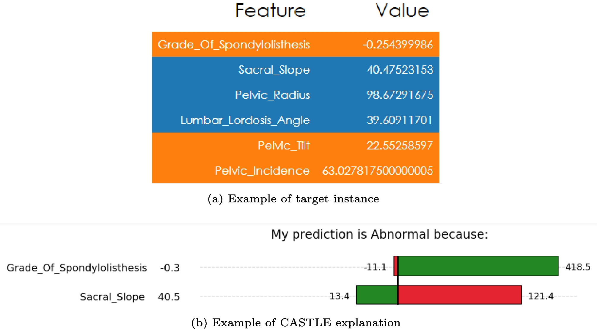
To show an example of its working, let us consider again the instance from the vertebral column datasetFootnote 2 (Fig. 1a). For simplicity, let us just consider the top two features: Grade of Spondylolisthesis and Sacral Slope. A possible cluster could be described in the form:

$$\begin -11.1 \le Grade\ Of\ Spondylolisthesis \le 418.5 \end$$

$$\begin 13.4 \le Sacral\ Slope \le 121.4 \end$$

As will be detailed later, clusters’ description can be used as an explanation only if the properties of purity, coverage, and overlap are enforced. Moreover, it is worth noting that the cluster’s representation as an axis-aligned hyper-rectangle is a necessary choice to favor the interpretability of explanations in the trade-off between expressive power and interpretability. For example, considering data distributed as a slanted line in a high-dimensional space, our description would be interpretable but it would include unnecessary volume; on the other hand, an elliptical description would be more accurate but not interpretable at all.

Fig. 2

The cluster alone does not provide much information about the prediction outcome. That is why you need to combine this piece of global knowledge to the local behavior of the model around the target instance, to provide a clear and comprehensive explanation. Figure 1b shows the result of CASTLE applied to the above example. The identified clusters are represented in the feature values range under the form of rules, which means the patient is labeled as “Abnormal” because his Grade of Spondylolisthesis level lies in the range \([-11.1, 418.5]\) and his Sacral Slope value lies in [13.4, 121.4]. Furthermore, the green and red areas show the supporting and opposing directions to the prediction, respectively. This means, should the patient Grade of Spondylolisthesis level increase, the likelihood of him being considered “Abnormal” would increase. While an increase in his Sacral Slope value would weaken the current prediction.

The overall explanation extraction process in CASTLE consists of two main phases:

1.

Preparation: one-time fitting of a clustering model which represents the global knowledge of the predictive model.

2.

Explanation: extraction of both global and local behavior of the classification model. Global behavior is retrieved by finding the cluster which most likely applied to the target instance, while local behavior is obtained by analyzing model’s outputs for instances in the neighborhood of the target.

Preparation Phase

The goal of the preparation process is to find a set of clusters grouping instances which share a common behavior and which are homogeneously classified by the predictive model. More in detail, the classification model \(f(\cdot )\) is used to obtain labels for data on which the model has been trained, which are the basis of its knowledge. Then, a clustering procedure aims to mine the knowledge acquired by the model, and representative points for each cluster (named pivots) are eventually pulled out and will be exploited by the explanation phase. The clustering procedure, through the identification of the axis-aligned hyper-rectangle which includes the cluster instances, enables the possibility to provide logic rules as a part of the explanations, which can be easily understood by humans. For this reason, not only should clusters respect the usual clustering properties (like low intra-variance and high inter-variance), as shown in Fig. 2, but they should also have the following characteristics:

High purity: The user expects the logic rule to be trustworthy and, hence, that every instance lying in the hyper-rectangle has the label specified by the rule (the same label as the target instance being explained). Given a cluster \(C_j\), its purity can be defined as the percentage of instances lying in \(C_j\) with the majority-class label.

High coverage: It is simple to obtain completely pure clusters, even in highly overlapped datasets, if we allow the clustering algorithm to not cover every instance (refer, for an example, to Fig. 2a). At the same time, it is simple to cover every instance if there are no purity restrictions (refer to Fig. 2a). In real-world scenarios, where there usually is no well-defined boundary between classes, it is necessary to handle a trade-off between purity and coverage: a high purity increases the user trust towards the explanation system, but the not-covered areas of the instance-space result in the inability to provide logic rules when required.

Low overlap: The area shared by clusters representing different classes must be as small as possible. As a matter of fact, the model’s behavior is uncertain in these areas, and that could jeopardize users’ trust towards the system. Figure 2c shows an example of overlap. Formally, overlap is defined as the mean of the Intersections-over-Unions (IoUs) between the clusters (axis-aligned hyper-rectangles) representing different classes. So, given a classification problem with s classes and, consequently, s cluster sets \(\mathbb ^0,\mathbb ^1,...,\mathbb ^\), overlap can be computed as follows:

$$\begin \begin overlap=\frac^|\mathbb _i||\bigcup _^\mathbb _j|}\\ \sum _^\sum __i}\sum _^\mathbb _j}IoU(C_w,C_z) \end \end$$

(2)

Once the appropriate cluster set is found, the last step of the preparation phase consists of extracting one or more representative points, called pivots, from each cluster. They will be exploited to retrieve the explanation in the following phase. A simple, yet efficient choice for pivots could be the clusters’ centroids. Note that this phase is totally absent in LIME, as it lays the foundation for the “global” understanding of the model, described in the following section. So, if on the one hand it adds overhead to the methodology, on the other hand, it allows for a complete and exhaustive explanation.

Explanation Phase

The explanation phase represents the core of the proposed methodology. Its aim is to extract a comprehensive explanation for the target instance outcome, basing both on the global and local behavior of the predictive model.

Fig. 3

Explanation phase: local behavior

The “global” understanding of the model is achieved by finding the cluster which is most likely applied to the target instance. This could be simply implemented by selecting the cluster whose centroid is closer to the instance. Once the target has been assigned to a cluster, the extraction of the rule consists of finding the axis-aligned hyper-rectangle that represents it (for example, you could select all the instances belonging to the target cluster and define the boundaries by computing the minimum and maximum value for each feature).

The process for understanding the local behavior of the model is shown in detail in Fig. 3. As a matter of fact, CASTLE and LIME share the same phases in this process, applied in a slightly different way. So, you can both get information about the main features contributing to the prediction, and also estimate how much the prediction is influenced by the proximity of the target instance to the pivots retrieved from the clusters.

Fig. 4

Example of the pivot-based space transformation

First of all, the neighbors of the target instance define its locality. They are commonly generated by random perturbation of the instance to be explained. Every neighboring instance generated is forecasted by the input black-box model, with the underlying concept being that we can reconstruct the model’s specific behavior within the vicinity established by these generated instances.

The novel idea of our approach is an instance-space transformation, named CAST, such that each feature represents the proximity of the target instance to a pivot. Let us consider a binary two-dimensional problem where instances are preliminarily divided into two clusters, and their centroid is the pivots \(p_0,p_1\). Given a target instance \(t=(x_0,x_1)\), it can be encoded into a new variable \(t'=(x'_0,x'_1)\), where \(x'_i = proximity(t,p_i)\) is a measure of similarity between t and the pivot \(p_i\). A simple example of a proximity function is as follows:

$$\begin proximity(t,p_i)=\frac \end$$

(3)

where \(d(t,p_i)\) is the distance between t and \(p_i\). Figure 4 shows an example of transformation using Eq. 3 as a proximity function. As you can see, red points in the new space are on the top-left region of the plot because they have a small proximity to pivot 1 and a big proximity to pivot 2, and vice versa.

Finally, the transparent model fitting phase consists in learning a transparent model (e.g., linear regressor, decision tree) on the neighbors, exploiting the black-box model predictions. In other words, the proposed model encapsulates the internal mechanisms of the black-box model within the proximity of the target instance. More precisely, the interpretable model, trained on modified data, calculates a weight for each pivot, signifying the extent to which the proximity of the target instance impacts the prediction. For instance, the output y(t) of a linear model can be expressed as follows:

$$\begin y(t) = \sum _}, \end$$

(4)

where t is the target instance, \(\mathbb \) the set of pivots, and \(w_p\) the learned weight for pivot p which represents its influence to the prediction.

It is worth noting that the space transformation has no impact on the behavior of the black-box model, as it was queried with the neighbors in the original space.

Furthermore, an additional interpretable model can be trained using the original neighbors, akin to the approach in the LIME framework. This helps in understanding the influence of data features on the local prediction. It can be insightful to view the output of the interpretable model fitted on CAST data as if it were a combination of gravitational forces acting on the target instance to guide it towards its predicted outcome, as depicted in Fig. 5. Each pivot, denoted as p, exerts an attractive force when its weight \(w_p\) is positive (indicating a positive contribution to the prediction), and conversely, a repulsive force when the weight is negative. The impact of each pivot is determined by both its weight and its proximity to the target instance: reducing the distance between the target instance and a positively weighted pivot enhances the likelihood of predicting the corresponding class. The resultant force represents a vector pointing towards the most supportive region for the prediction y(t), with its magnitude signifying the predicted value.

Fig. 5

Explanation vector as a sum of pivot contributions to the prediction

How to Choose Pivots

When performing a transformation of the instance space, it is crucial to guarantee the preservation of information from the original space in the new one. From a mathematical standpoint, this entails ensuring the injective property of the space transformation: every element in the transformed space corresponds to at most one element in the original space. Achieving this requires the involvement of an appropriate number of pivots in the transformation process. To be more specific, it is imperative to select a minimum of \(d+1\) pivots (where d represents the dimensionality), as illustrated in Fig. 6 through a simple two-dimensional example.

Fig. 6

a In a two-dimensional space featuring three distinct pivots, if the Euclidean distance is employed as the proximity metric, the instance denoted as t can be transformed into \(\hat=(d_1, d_2, d_3)\). The presence of three non-aligned pivots ensures that \(\hat\) corresponds exclusively to the original instance t, as it is the solitary point of intersection among three circles centered on the pivots and having their respective distances as radii. b When only two pivots are selected, the transformed instance \(\hat=(d_1, d_2)\) matches with two distinct points, namely, \(t_1\) and \(t_2\), which represent the intersections of the two circles formed by the selected pivots. This scenario may result in a potential loss of information

The choice of pivot selection strategy within the system may vary depending on the user involved. On one hand, the level of comprehensibility required by the audience differs based on whether they are end-users or considered “expert” analysts, as discussed in [27]. End-users may primarily seek an understanding of why the model made a specific prediction, such as why their loan application was not approved. Conversely, expert analysts may aim to scrutinize the model’s vulnerabilities and seek improvements, such as identifying potential biases stemming from the training data. On the other hand, the level of familiarity with the model also differs among these user groups: developers possess knowledge about the training process and can access model-related data, while end-users are limited to interacting with the model through its interface.

CASTLE provides users with access to training data and knowledge about the training process, such as developers and expert analysts, with the means to thoroughly investigate the dynamics of the model. This investigation involves the analysis of both the supporting directions and the relevance values of the chosen pivots. Expert analysts with data access can exercise control in extracting pivots by leveraging clustering techniques and their domain expertise. This approach enables them to select pivots that ensure a significant separation between classes within the transformed space. For instance, there are several strategies based on pivot selection metrics that can be effectively employed to enhance pivot selection and subsequently improve nearest neighbor or range query searches, as elaborated in [37].

When an end-user has data access but lacks the expertise or time to manually choose pivots, an automated explanation process can be facilitated using a random selection strategy. It has been empirically demonstrated that this approach does not negatively impact performance. In the broader context, for end-users who have neither data access nor training information, a fully automated procedure can be employed, where pivots are selected through random perturbation of the target instance.

CASTLE on Big Data Architecture

The process has been carried out with a bottom-up approach, by identifying the main steps and entities that characterize an explanation process and connecting them together to create the final framework that relies on big data technologies. This is mainly because of their modularity: in fact, it is easily replace the underlying machine learning model or just as easily replace the interpretation method. These are the reasons why it is possible to create a generalizable architecture, which can just as easily be extended to embrace more and more algorithms as the research goes on. The milestone steps of the post hoc local explanation process are as follows:

1.

Get the class predictions for your data through a black-box ML algorithm.

2.

Generate a neighborhood around the target instance you want to provide an explanation for.

3.

Make the black-box model (used in the first step) predict the class label for the new instances.

4.

Fit a simple, transparent model on the newly generated neighbors to get an explanation of the model behavior in the locality of the target instance.

By following this schema, it was possible to implement the framework shown in Fig. 7. For the sake of readability and clarity, only the main methods (directly involved in the explanation process) are displayed. In the following sections, each entity represented in the architecture will be discussed.

Fig. 7

General framework for our method

The first package, named data, contains the entities to handle different data (TextData, ImageData, or TabularData) from an external source. Successively, model connectors are defined in order to implement the independence of the explainer from the specific black-box classifier. In particular, Model is \(<interface>\), which provides the method predict() to get the label predictions of the black-box model for the instances generated in the target instance neighborhood while ScikitConnector and SparkMLConnector are respectively the connector for Python scikit-learn machine learning library and MLLib from Apache Spark for integrating whichever ML model. The explainer package, then, represents the core of the whole explanation process, whose main entities are as follows:

Explainer

This is the general interface that allows to produce an explanation for the behavior of a black-box model. As you can see from the architecture Fig. 7, it makes use of the model it is going to explain, and of course the data to retrieve all the information it needs. Once the explainer has computed all the steps, it instantiates an Explanation object, which will be analyzed later. In particular, it is possible to distinguish between global and local explainers, basing on your scope. GlobalExplainer can be used for those techniques, whose goal is to provide a global explanation of the whole ML model, so as to understand the entire logic behind it. On the other hand, LocalExplainer can be exploited to produce an explanation for a target instance, without having to go into the details of the whole model understanding.

Table 2 Datasets characterization LIMEExplainer

This is the main class for the implementation of LIME [18]. Being a local explanation strategy, it expands LocalExplainer and provides an explanation for a target instance. According to the type of data you are going to handle, you can either use LIMETextExplainer, LIMEImageExplainer or LIMETabularExplainer. This is the class responsible for the neighborhood generation process and the definition of the locality of the target instance. Once the needed computations have been completed, it calls the method explain_instance_with_data(), provided by LIMEBase, to generate the explanation.

LIMEBase

This is the final step of the explanation process, where the simple, transparent model is fitted on the neighborhood data, previously labeled by the classifier, to generate an interpretable explanation for the target instance outcome.

CASTLEExplainer

It implements another local explanation methodology. Its inner working is similar to LIME, but it additionally exploits global knowledge about the data, through a clustering technique, to provide more information about the outcome.

Finally, the explanation package contains the possible explanation forms (i.e., rule, example, or FeatureImportance) you can get from an explainer.