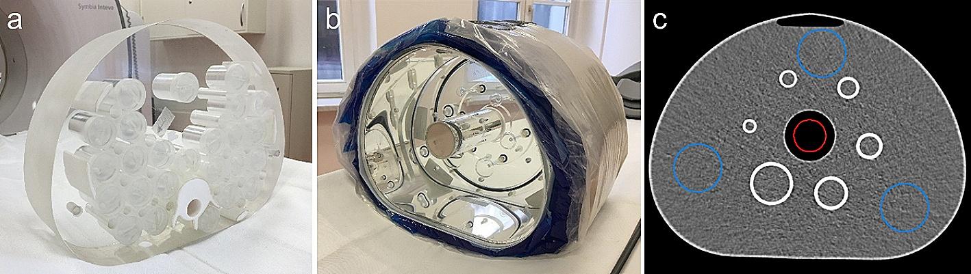
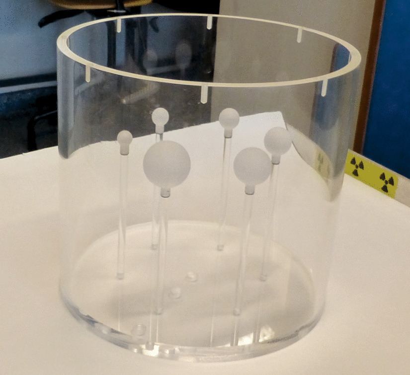
Phantom measurement

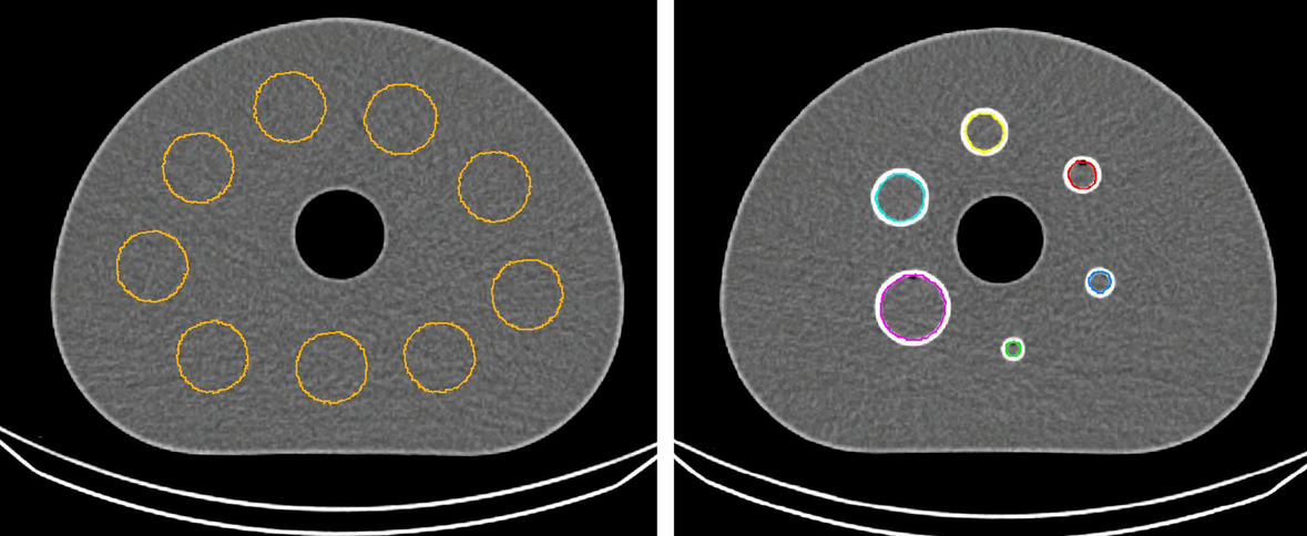
Phantom measurements, using the NEMA IEC body phantom, were conducted to assess the general feasibility of fast SPECT imaging over an extended field-of-view, using a projection time of 5 s in combination with the clinically used imaging and reconstruction parameters. Additionally, the threshold for a reasonable lesion volume should be determined for this study. All six spheres (26.52, 11.49, 5.58, 2.57, 1.15 and 0.52 ml) were filled with an activity concentration of 1046 kBq/ml and the background was filled with 65 kBq/ml, resulting in a sphere-to-background ratio of 16:1. This high ratio was chosen because mainly bone lesions were evaluated, which are typically located in a low background activity. The sphere recovery coefficients were determined by dividing the respective average activity concentration as measured in the SPECT by the known activity concentration. The background activity was not considered in these calculations. To measure the activity concentration in the spheres, two methods were used, a CT-based and a threshold-based method. In the CT-based method, spherical volumes-of-interest (VOIs) with the known sphere diameters were placed on the high-resolution CT images (voxel size 1.2 × 1.2 × 1.2 mm3) and thereafter transferred to the SPECT images to collect the mean activity concentration in the VOIs. However, defining bone lesions in clinical low-dose CT images may be challenging. Thus, in the second method, the spheres were delineated directly on the SPECT images using a threshold-based method originally evaluated on PET images [21]. In this method, a spherical VOI with a 12 mm diameter was employed with the sphere center being placed at the maximum activity concentration of each lesion. A 30%-isocontour of the average within this VOI was then used to obtain the respective lesion contours.

Patients

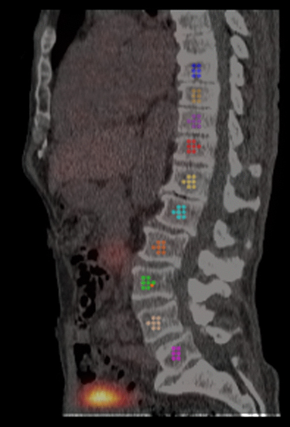
This study is based on five patients with mCRPC, who underwent their first cycle of 177Lu-PSMA-I&T therapy. PSMA expression was verified prior to therapy via 18F-PSMA-1007 PET/CT imaging. All patients gave written consent to undergo radioligand therapy. All data were irreversibly anonymized before evaluation. The study was performed in a retrospective manner with approval from the local ethics committee (project number: 22-0552). Four patients were administered a therapeutic activity of 7417 ± 22 MBq, while one patient received 8925 MBq 177Lu-PSMA-I&T due to diffuse bone metastases. For kidney protection, the patients received an infusion of 1000 ml of NaCl shortly after therapy and were instructed to ensure adequate hydration. SPECT/CT measurements were acquired at 19 ± 1 h, 42 ± 1 h, 66 ± 1 h and 170 ± 2 h p.i (days 1, 2, 3 and 7 in the following) over three bed positions beginning from the eyes downward. Within the clinical protocol at our department, no measurements before 1 day p.i. are acquired for logistic reasons and patient comfort on the day of therapy [17]. The acquisition time for the complete SPECT field-of-view of about 1.2 m was approximately 15 min. In four patients, metastases were mainly localized in the skeleton, whereas one patient predominantly had lymph node metastases.

Image acquisition and reconstruction

Quantitative SPECT images were acquired for both, the patients and the phantom, on a dual-headed Siemens Symbia Intevo T16 SPECT/CT (Siemens Healthineers, Erlangen, Germany) using the upper photopeak of 177Lu (208 keV, width: 15%) with scatter windows (170 keV, width 15% and 240 keV, width 10%) and the medium-energy low-penetration collimator. According to the standard clinical protocol, the matrix size was set to 128 × 128 pixels. 64 projections per detector head were acquired in auto-contour mode, each with an acquisition time of 5 s. Quantitative SPECT images were reconstructed with Hermes Hybrid Recon-Oncology 4.0 (Hermes Medical Solutions, Sweden), using a calibration factor of 7.9 cps MBq−1, a maximum-a-posteriori ordered-subset expectation–maximization (MAP-OSEM) algorithm with 16 iterations, 8 subsets, and a quadratic penalty with a factor of β = 0.001. Quantitative reconstruction included CT-based attenuation correction, a Monte Carlo-based scatter correction, and resolution modeling [22, 23]. The CT measurement was conducted with 110 keV tube voltage and with CareDose enabled using a reference current of 15 mAs and a slice thickness of 3 mm.

Image processing

Further processing of the reconstructed clinical SPECT images was continued in PMOD (Version 3.609, PMOD TECHNOLOGIES LLC, Switzerland). The lesions were segmented day-wise according to the iso-contour method described in the phantom section. Kidney VOIs were drawn manually slice by slice on the CT images. The mean activity concentration and the VOI volume were extracted from PMOD for each lesion and kidney. Further, to correct absorbed doses for the individual VOI mass, for each VOI the corresponding Hounsfield Unit (HU) was extracted from the CT data and converted into an average VOI density. In order to convert the mean HU of each VOI into density values, a calibration curve was employed, which was previously established via a Gammex Tissue Phantom [24]. More Precisely, the known densities of 11 tissue-mimicking materials were plotted against the HU as measured for the employed CT system and fitted by a linear model, resulting in ρ = 7.94E−5 ± 0.34E−5*HU + 9.64E−1 ± 0.18E−1. This provides a formula to convert the mean HU of each lesion or kidney VOI into a mean density. The respective plot with linear fitting is shown in Additional file 1. In total, 43 lesions, five of which were soft tissue and the rest bone lesions, and 10 kidneys were segmented.

Fit models and model selection

In MATLAB (v2011-R2016), the absorbed dose of each VOI was calculated. In order to obtain the time-integrated activity (TIA), the TAC model was fitted to the VOI data using a nonlinear-least-squares algorithm and integrated from zero to infinity. For the determination of the reference model for both, kidneys and lesions, all four available TPs (1, 2, 3 and 7 days p.i.) were included and the ‘best’ fit function was evaluated. All models proposed by Hardiansyah et al. were considered, which were originally evaluated for kidney biokinetics [19]. The goodness-of-fit was checked by visual inspection, the coefficient of variation (CV) in percent and the sum of squared errors (SSE) averaged over all lesions [19, 20, 25]. The CV includes the standard error of the fit parameters which should optimally be small. CVs less than 25% usually indicate that the parameter estimates are precise. Since all tested fit functions have the same degrees of freedom, the SSE provides information about the quality of the model: the smaller the SSE, the smaller the difference between the data point and model estimate.

After a first selection process, which removed all functions for which the fitting either failed or had coefficients of variation (CV) larger than 100%, the following functions were further considered for model selection:

For lesions:

$$f_}}} \left( t \right) = A_ e^}}} + \lambda_}}} } \right)t}} ,$$

$$f_}1,}\upgamma }} \left( t \right) = A_ }e^}}} + \lambda_}}} } \right)t}} + A_ \left( }} \right)e^}}} } \right)t}} \;}\;}\;\gamma ,$$

$$f_}1,}}}} \left( t \right) = A_ \gamma e^}_}}} + \lambda_}}} } \right)t}} + A_ \left( \right)e^}}} } \right)t}} \;}\;}\;\lambda_}}} .$$

For Kidneys:

$$f_}}} \left( t \right) = A_ e^}}} + \lambda_}}} } \right)t}} ,$$

$$f_}1,}\upgamma }} \left( t \right) = A_ }e^}}} + \lambda_}}} } \right)t}} + A_ \left( }} \right)e^}}} } \right)t}} \;}\;}\;\gamma ,$$

$$f_}1,}}}} \left( t \right) = A_ \gamma e^}_}}} + \lambda_}}} } \right)t}} + A_ \left( \right)e^}}} } \right)t}} \;}\;}\;\lambda_}}} ,$$

and

$$f_}2,}1}} \left( t \right) = A_ e^}}} + \lambda_}}} } \right)t}} + }_ e^}}} } \right)t}} \;}\;}\;A_ ,$$

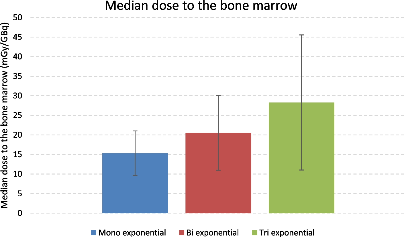
with the activities A0 (A (t = 0)) and A1, the factor γ (0 < γ < 1), the physical decay constant λphys = 4.34E−3 h−1 of 177Lu and the biological clearance rate λbio. The mono-exponential function is characterized by two free parameters, A0 and λbio, whereas the bi-exponential functions use additional parameters γ and A1. For all bi-exponential functions, one parameter each is considered as a population-based, shared parameter. They are estimated using the Jackknife method [26, 27]. Within this approach, the shared parameter is determined for each patient by fitting the respective bi-exponential function to all lesions from the patient cohort, with all lesions from the patient under consideration being excluded. An exception was made for the kidney γ-factor, which has already been reported to be 0.963 ± 0.004 for a large population of 13 177Lu-PSMA-I&T patients [19]. This procedure reduces the number of free parameters for the bi-exponential functions to two. Out of the functions presented above, the best-fit function was chosen to be the one with the smallest CV and SSE separately for lesions and kidneys.

Biologically effective dose calculation

The absorbed dose was estimated following the MIRD scheme with the assumption that the source region is equal to the target region due to the short range of beta radiation from the 177Lu decay [28]. Using the time-integrated activity (TIA), the absorbed dose D can be determined by

with the S-factor being the mean absorbed dose to the target region per radioactive decay in the source region. The used lesion S-value of 2.33E−5 Gy MBq−1 s−1 (for 1 g tumor) was derived from OLINDA/EXM with the approximation of unit density spheres corrected for the lesion-specific average density [29]. The kidney S-value of 7.38E−8 Gy MBq−1 s−1 (for 310 g kidneys) was likewise corrected for the patient-specific kidney mass [30].

In the next step, the BED was derived using the equation

with the relative effectiveness RE. For radioligand therapy, the RE can be written as

$$} = 1 + \frac \cdot G,$$

where α and β are radiosensitivity constants defined by the tissue and G is called the Lea-Catcheside factor [31]. Assuming a mono-exponentially decreasing activity in the source organ, G is expressed as

$$G = \frac}}} }}}}} }} ,$$

where λeff = λphys + λbio are the effective clearance rate of the source region and µ is the repair rate of the tissue. In case of a bi-exponential clearance, the Lea-Catcheside-factor is given by

$$G = \frac^ }} \left( } \right)}} + \frac a_ }} + \lambda_ } \right)\left( } \right)}} + \frac a_ }} + \lambda_ } \right)\left( } \right)}} + \frac^ }} \left( } \right)}}}} }} }} + \frac }} }}} \right)^ }}$$

with λ1 = λeff and λ2 = λphys [32]. The so-called dose rate fraction coefficients a1 and a2 are hereby determined as follows:

$$a_ = \frac \cdot \gamma }}}}} \left( \right)}}\;}\;a_ = \frac \left( \right)}}}}} \left( \right)}} .$$

The α/β-ratio of tumors was set to α/β = 3.1 Gy as reported by Wang et al. for mCRPC [33]. For the repair rate, a repair half-life Tµ of 1.9 h was used [33]. The respective kidney parameters were α/β = 2.6 Gy and Tµ = 2.8 h [34].

In addition to lesion-wise calculation, total tumor dose and respective BED were determined by averaging the activity concentrations and summing the tumor masses of all lesions of one patient.

Data evaluation

In order to evaluate the impact of different time samplings, the BED was calculated for all lesions and kidneys with different sampling schedules and compared to the reference model. The fit model determined for the reference was also used for all other time samplings. Since in many countries every SPECT/CT measurement has to be performed on an outpatient basis and every way back and forth from the hospital may be challenging for the patients, the following sets of data points were investigated: days 1, 2, 3 versus 2, 3, 7 versus 1, 2, 7 versus 1, 3, 7 with all including three TPs and days 1, 2 versus 1, 3 versus 1, 7 comprising two TPs. All possible variations of three TPs were used while for two TPs, it is assumed that patients stay at the hospital until 1 day p.i. and just have to come in again once for the second measurement.

The performance of these time samplings regarding dosimetry was evaluated by Bland–Altman plots and relative deviations (RD) from the respective reference model:

$$} = \frac} - }_}}} }}}_}}} }} \cdot 100\% .$$

Thus, positive RD indicates an overestimation of the BED compared to the reference, and negative RD an underestimation. In order to assess the total deviation of all BEDs from the reference model within one sampling schedule, the absolute deviation (MD) was calculated and averaged over all lesions or kidneys.