NEMA IQ phantom

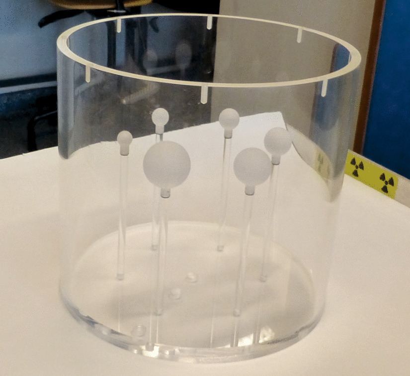
The National Electrical Manufacturers Association (NEMA) Image Quality (IQ) phantom featuring six fillable spheres with inner diameters of 10 mm, 13 mm, 17 mm, 22 mm, 28 mm, and 37 mm was filled with Lu-177 activity concentrations of 6.41 MBq/mL for the spheres and 0.53 MBq/mL for the background. As such, a 12.1 contrast ratio was achieved between spheres and the background to replicate clinical lesions. With these concentrations, a High-count (HC) scan was first emulated, followed by nine other scans with the same sphere-to-background ratio but with decreasing activity concentrations due to physical decay. As a result, the last scan was considered a Low-count (LC) scan with an activity concentration of 0.8 MBq/mL for the spheres and 0.06 MBq/mL for the background.

Conventional SPECT/CT imaging

Conventional SPECT/CT imaging was performed with a dual-head Siemens Symbia T16 SPECT/CT system, equipped with medium-energy general-purpose parallel-hole collimators. Acquisition parameters of the CT scan were set to 130 kV, 30 mAs, and \(0.97 \times 0.97 \times 5\hbox ^3\) voxel size while the SPECT scanning protocol followed the protocol described by Marin et al. [8] with the following parameters: a \(128\times 128\) matrix, voxel size of 4.79 mm, 32 views with 30 s per view, and an energy window centered at the 208 keV photopeak (with a 20% width) combined with a lower scatter window (with a 10% width). The projection data were decay and scatter corrected and reconstructed using Ordered Subsets Expectation Maximization (OSEM) [9]. To optimize the reconstruction protocol such that sphere-to-background ratios were as close as possible to the true ratio while keeping the noise level as low as possible, the number of iterations and subsets were gradually increased (4i4s, 8i8s, 16i16s and 24i16s) with 16 the highest possible number of subsets. In addition, default post-smoothing was performed with a Gaussian filter of 1 mm Full width half maximum (FWHM), with additional filtering being considered to further reduce the noise if necessary.

3D CZT SPECT/CT imaging

The ring-like CZT system is a 12-headed Veriton SPECT/CT system, manufactured by Spectrum Dynamics. This system comes with an integrated collimator made out of Tungsten and optimized for low-energy photons (70 to 200 keV). As it is not an externally applied collimator, it cannot be changed and all imaging needs to be done with this collimator. Since the energy range of this system is limited to 200 keV because of the limited stopping power of the 6 mm CZT crystal, the energy window was centered at the lower 112.9 keV photopeak (20% width) of Lu-177. Triple energy window (TEW) scatter correction was used with the lower scatter window centered at 90.3 keV (20% width) and the upper energy window at 135.5 keV (20% width). The main and scatter windows were fixed by the manufacturer, such that no further optimization was feasible. The StarGuide from GE Healthcare is a similar 3D CZT SPECT/CT and has a crystal of 7.25 mm. It can therefore utilise the 208 keV peak. A full analysis of this system for Lu-177 was performed by Danieli et al. [10].

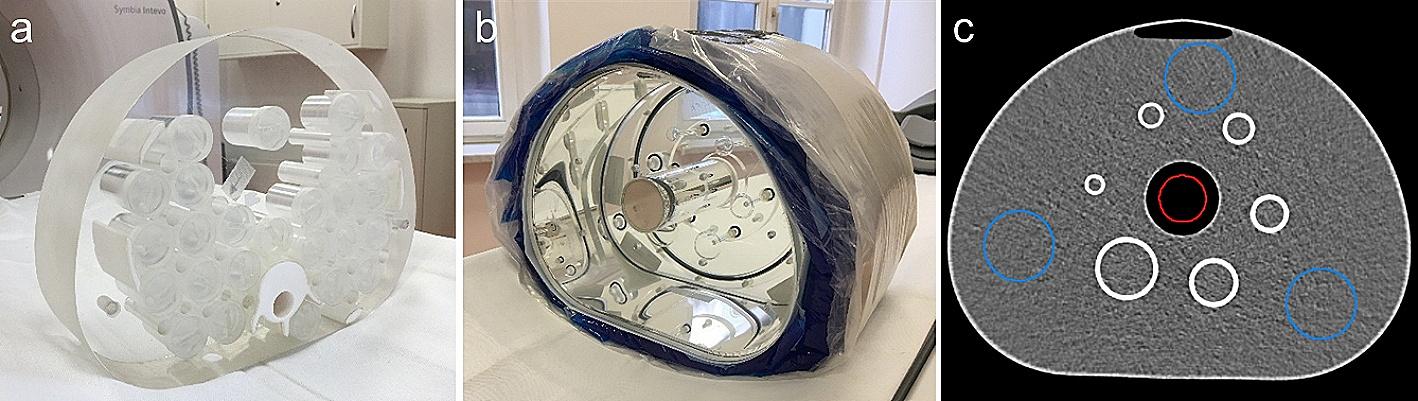
The phantom was scanned with auto-contouring activated, as this is also how patient images are acquired. In addition, using auto-contouring increased the total number of counts by 10.6% compared to not using auto-contouring. To perform auto-contouring, aluminum foil was placed around the NEMA IQ phantom. This was done to prevent any collisions with the detector heads, as the auto-contouring system relies on capacitance proximity. Without the aluminum foil, the Veriton SPECT/CT was not able to detect the plastic edge of the phantom.

The clinical protocol was based on the protocol by Vergnaud et al. [11] where it was concluded that applying TEW scatter correction gave the highest recovery coefficients compared to including a detector response model in the reconstruction. As detector response modeling and scatter correction cannot be combined, the latter was chosen. For the attenuation correction, a CT scan was performed at 120 kV, 21 mAs and \(1.27 \times 1.27 \times 2.5\hbox ^3\) voxel size. A voxel size of 2.46 mm was chosen for all SPECT reconstructions while reconstructed images were by default post-smoothed with a Gaussian filter of 3 mm FWHM. To optimize the reconstruction in terms of sphere-to-background ratios and noise level, the number of iterations was gradually increased (5, 10, 25, 50 and 100) while 2 subsets were chosen for each number of iterations to keep the number of subsets as low as possible to ensure convergence.

Once the optimal reconstruction protocol was determined, the impact of further reducing the acquisition time on image quality was also assessed. For this purpose, additional phantom scans with a shorter scanning time were obtained from the phantom data with 6 min of acquisition time by reducing the list mode data based on a shorter virtual scanning time. These virtual scans with a reduced number of counts were combined with the scans acquired with lower activity concentrations and compared to the 6 min scan which was considered as the reference high-count (HC) scan.

SPECT image characteristics using the NEMA IQ phantomImage calibration

To calibrate the SPECT system, nine spheres (each with 35 mm diameter) were drawn at different locations in the uniform region of the NEMA IQ phantom and used to compile one larger background Volume of Interest (VOI) (see Fig. 1) to measure the total number of counts \(C_\) in this background region.

For the conventional system, the calibration factor \(Q_\), expressed in [cps/MBq], was calculated by Eq. 1 with \(C_\) the total number of counts in the predefined background, \(A_\) the true decay-corrected activity in that specific VOI as measured with the radionuclide calibrator and T the total acquisition time.

$$\begin Q_ = \frac}\cdot T} \end$$

(1)

For a setup of 32 views per head and 30 s acquisition time per view, the total acquisition time equals \(T = 32\cdot 30\,\text \cdot 2\) since two detector heads were used. Because \(C_\) is defined as the total number of counts measured in all voxels of the VOI, the calibration factor \(Q_\) depends on the acquisition time, reconstruction settings (voxel size and number of iterations and subsets) and amount of post-smoothing since all these factors can impact the total number of reconstructed counts. Therefore, a calibration factor should be determined for each predefined acquisition and reconstruction protocol.

For the 3D CZT system, the base unit for measurements is \(\frac\), which is a proportional unit that considers the isotope’s physical characteristics for the detector sensitivity correction map and the time each voxel in the image was measured according to the system model. The latter is a result of the swiveling motion of the detectors, which makes acquisition time spatially dependent. The system calibration factor \(Q_\) converts this proportional unit to Bq/mL which has the advantage that the calibration factor is independent of the acquisition time and voxel size. However, the system calibration is still dependent on the reconstruction parameters as these directly influence the activity concentration measured by the system. As a result, the calibration factor \(Q_\) of the 3D CZT system is given by Eq. 2, with \(C_\) the total number of counts in the background VOI which is proportional to Bq/mL, \(A_\) the true activity concentration in the background VOI expressed in MBq/mL and \(10^6\) a correction factor to account for the difference in units.

$$\begin Q_ = \frac}\cdot 10^6} \end$$

(2)

Fig. 1

Delineation of the background VOI (left) and the spheres (right) on the corresponding CT image

Based on Eqs. 1 and 2, the relative uncertainty of the calibration factor Q is a combination of the uncertainty of the relative uncertainty on the radionuclide calibrator measurements \(A_\) and the background count measurements \(C_\). This is given in Eq. 3. This dependence is visualized in the total uncertainty scheme in Fig. 3.

The relative uncertainty on the background count measurement was defined as the standard deviation divided by the average value of \(C_\), calculated over all ten scans (see Sect. ). The relative uncertainty on the radionuclide calibrator measurements was considered equal to the uncertainty of the activity measurement of the calibration vial.

$$\begin \left[ \frac\right] ^2 = \left[ \frac)}_}\right] ^2 + \left[ \frac)}}\right] ^2 \end$$

(3)

Image quality assessment

To assess image quality, only the HC and LC scans were used. Each fillable sphere within the NEMA IQ phantom was defined on the corresponding CT image using a region-growing algorithm, with the edge of each sphere serving as a boundary (see Fig. 1). These VOIs were then transferred to the SPECT data. Due to the limited spatial resolution of the SPECT data, the two smallest spheres were excluded from the analysis.

For the 3D CZT and conventional SPECT/CT system, various reconstruction protocols were then considered. These protocols were evaluated based on the measured sphere-to-background ratios using the mean values of the spheres relative to the mean value of the composite background VOI, as a function of the background Coefficient of Variation (CoV). The goal was to identify the reconstruction settings that matched the true sphere-to-background ratio of 12.1 as closely as possible while keeping the background CoV (noise) as low as possible.

Image resolution

A matching filter method was used to estimate the spatial resolution of the high-count (HC) SPECT images that were acquired and reconstructed according to the optimized clinical SPECT imaging protocol [12].

For this approach, a template of the NEMA IEC phantom was generated starting from the HC SPECT/CT scan. First, the different spheres, the background and the lung compartment were delineated based on the corresponding CT data using region growing. For the Siemens Symbia PET/CT data, both the template and the HC SPECT scan were resampled to match the voxel size of the Veriton (2.46 mm), as the original voxel size of 4.79 mm resulted in undersampling of the VOIs from the CT image when transferred to the SPECT image. Next, the value of the background compartment of the template was set to the mean value of the background VOI of the HC SPECT image while the value of the spheres was set to 12.1 times the background value and the value of the lung compartment was set to zero. This was done to allow the template to match the SPECT scan as much as possible. Subsequently, the template was smoothed with a 3D isotropic Gaussian filter using different FWHM values, ranging from 0 to 18 mm.

For every FWHM, the Peak Signal-to-Noise Ratio (PSNR) was calculated using the HC SPECT scan as a reference. First, the Mean Squared Error (MSE) was computed between the reference HC SPECT image and the smoothed template image for all image slices containing the spheres. Next, the PSNR was calculated as the ratio between the maximum uptake value of the reference HC SPECT image and the MSE. This ratio is then converted to dB by Eq. 4.

$$\begin PSNR = 20\,\log _\left( \frac}\right) \end$$

(4)

If smoothing of the template with a specific FWHM provided a voxelwise better approximation of the reconstructed HC SPECT image, the MSE would be lower for this FWHM and the corresponding PSNR higher compared to template images with a different degree of smoothing. To determine the FWHM resulting in the highest PSNR, the PSNR curve was approximated by a 2nd-order function in the relevant range and the FWHM corresponding to the highest PSNR value was determined by finding the root of the function. This FWHM was then considered the most representative value for the spatial resolution of the reconstructed SPECT image (Fig. 2).

Fig. 2

Axial view of the Veriton high-count SPECT scan of the NEMA IQ phantom, reconstructed with the optimized clinical protocol and its corresponding template for the same color window (left). Axial view of the Symbia high-count SPECT scan and its corresponding template for the same color window (right)

Dose uncertainty analysis

For clarification, a brief overview is given of the dosimetry uncertainty model used for this study. For more details, we refer to the EANM guideline on the uncertainty analysis for molecular radiotherapy absorbed dose calculations [7]. For \(\beta\)-emitters such as Lu-177, the Medical Internal Radiation Dose (MIRD) formalism defines the self-absorbed dose \(\overline\) in OAR and tumoral lesions as the product of the time-integrated activity \(\tilde\) and the corresponding tumor or OAR S-factor. The relative uncertainty of the absorbed dose \(u(\overline) / \overline\) can therefore be calculated by Eq. 5, where the last term is the covariance term.

$$\begin \left[ \frac)}} \right] ^2=\left[ \frac)}} \right] ^2 + \left[ \frac)}} \right] ^2 + 2 \frac,S)},S)} \end$$

(5)

This equation can be expanded to Eq. 6. Here, Q represents the calibration factor and is calculated as mentioned in Sect. .

$$\begin \begin \left[ \frac)}} \right] ^2&= \left[ \frac \right] ^2 + \left[ \frac} \right] ^2 + \left[ \frac \right] ^2 - \frac \frac u^2(V) + |c_2|^2 \left[ \frac \right] ^2 \\&\quad -2\frac \left( \frac-\frac \right) u^2(V) \end \end$$

(6)

The volume uncertainty u(V) is calculated as in Eq. 7. Here, d is the equivalent diameter of the VOI and the uncertainty of this diameter is a combination of the voxel size a and the resolution quantified by the corresponding FWHM, as shown in Eq. 8. The S-factor uncertainty u(S) is directly proportional to u(V) as given in Eq. 9 with \(c_2\) a fitting constant of the S-factor.

$$\begin \left[ \frac \right] ^2= & \left[ 3\frac \right] ^2 \end$$

(7)

$$\begin = & \frac + \frac^2} \end$$

(8)

$$\begin \left[ \frac \right] ^2= & \left[ c_2\frac\right] ^2 \end$$

(9)

The uncertainty of the recovery coefficient u(R) can be calculated by Eq. 10, assuming that b are adjustable parameters of the recovery coefficient function, \(\textbf_}\) is the vector containing the partial derivatives of the first order of R to b and \(\textbf_}\) is the covariance matrix that includes uncertainties of the fitting parameters b and u(V).

$$\begin \left[ \frac \right] ^2= \textbf_}^T \textbf_} \textbf_} \end$$

(10)

The count rate uncertainty \(\) of the selected VOI at scan i, is calculated as in Eq. 11 with \(\) the error function.

$$\begin \left[ \frac \right] ^2 = \left[ \frac\frac\right] ^2 \end$$

(11)

For clarification, the dependency of the absorbed dose on different factors is also visualized in Fig. 3.

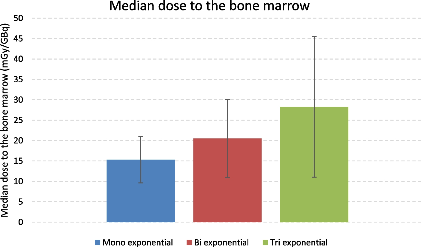
It can be seen that the uncertainty associated with fitting the time-activity curves is omitted from the equations. Our current clinical practice involves Lu-177 QSPECT/CT imaging at two time points, 20 h and 168 h post-injection. Using a mono-exponential model for estimating the effective half-life, induces no uncertainty on the estimated effective half-life and initial activity.

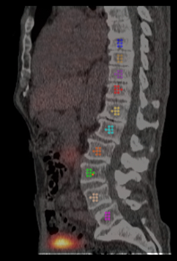
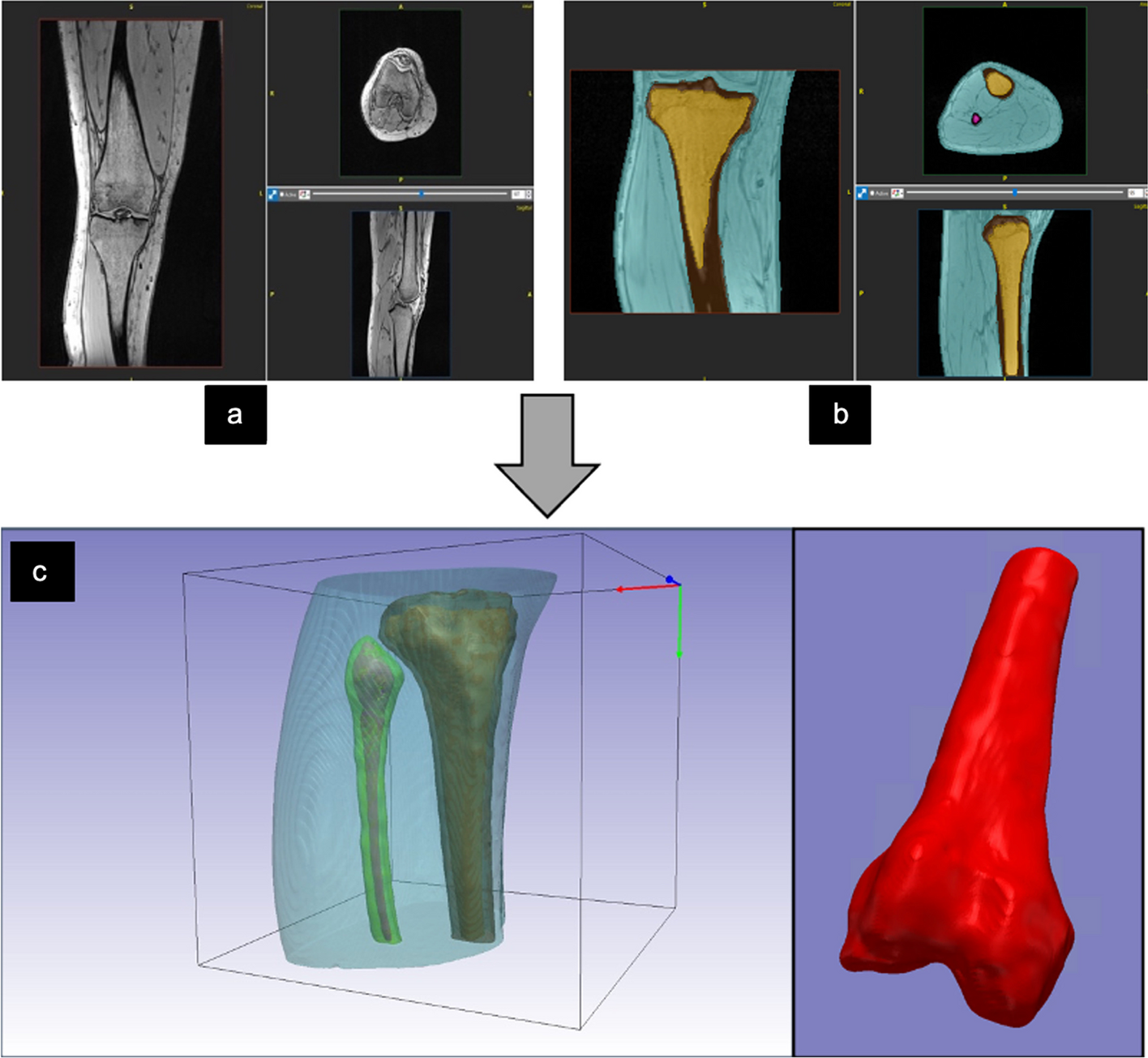
The volumes of kidneys and different tumoral lesions were estimated based on patient data to translate the impact of the dose uncertainties to clinically relevant lesions and organ volumes. 27 QSPECT/CT scans were taken on both systems from 13 patients treated with Lu-177-PSMA-617. The left and right kidneys are delineated on all images and the mean volume and counts are used to make an average single kidney. For the tumoral estimates, five lesions were used that were visible on CT. All kidneys and tumoral lesions were delineated on the CT data using a region-growing algorithm to estimate the organ and lesion volume and to apply the appropriate recovery coefficient. However, for a lung metastas is that was also included, the CT-based delineation was adjusted based on the SPECT data to account for the additional smoothing because of breathing motion.

Next, the time-integrated activity coefficients (or residence time) of Lu-177-PSMA-617 in each of the lesions and kidneys were estimated by fitting a mono-exponential model through the two time points and dividing the area under the curve with the total injected activity. By fitting S-factor data against mass, a suitable S-factor was determined [13].

Fig. 3

Flow diagram that shows the propagation of uncertainty