SPECT/CT systems

Two dual-head SPECT/CT systems, namely a Symbia T6 (referred to as Symbia) and a Symbia Intevo 6 (referred to as Intevo; Siemens Healthineers, Germany), both equipped with 9.5-mm-thick NaI(Tl) crystals and medium-energy low-penetration collimators were used.

In addition to the 177Lu photopeak (208 keV, 20%), lower and upper scatter windows (10% each), three additional energy windows were added to monitor the wide-spectrum count rate (18–680 keV), as previously described [8].

Phantom and patient acquisitions

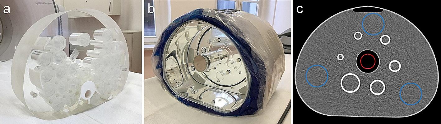
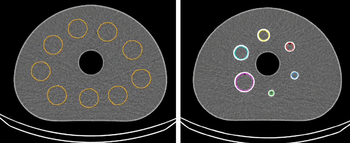
A NEMA 2012/IEC 2008 phantom (Biodex Medical Systems, USA) was customised with a similar geometry as the one described in [8]. A large saline bag (500 mL, 50 × background activity concentration) was placed right anteriorly to simulate a large liver lesion and a smaller one (250 mL, 10 × background activity concentration) left posteriorly to simulate a kidney (Table 1). Twenty acquisitions were performed with an initial total 177Lu activity of 20.75 GBq on the Intevo system. Phantom acquisitions were performed consecutively with only detector 1 activated and with both detectors activated [8]. All acquisitions were performed with a total number of 96 projections (10 s per projection for the first 13 acquisitions and then 20 s per projection for the seven remaining; 128 × 128 matrix; 4.8 mm pixel). SPECT acquisitions were followed by low-dose CT acquisitions (110 kVp, 70 mAs).

Table 1 NEMA phantom initial 177Lu activity distribution

Data of 14 patients enrolled in our prospective clinical trial of personalised PRRT (NCT02754297) were selected to gather a large range of average observed wide-spectrum count rate (Table 2) [2]. Day-1 QSPECT and Day-3 QSPECT were acquired at 23.3 ± 1.2 and 70.3 ± 0.7 h, respectively, following 177Lu-octreotate injection on the Symbia system. Acquisitions were performed with both detectors activated, as described above. The time per projection on Day 1 was either 15 or 20 s, while it was systematically 20 s per projection on Day 3.

Table 2 Patients quantitative SPECT data

The observed count rate was evaluated per projection and per acquisition to exclude saturated (i.e. non quantifiable) phantom data from further studies. An acquisition was considered as saturated if some plateau or abrupt normal variations were observed on the count rate versus projection graph [8].

Data reconstruction

Projections were reconstructed using SPECTRA Quant (MIM Software Inc., USA) with ordered subset expectation maximisation (four iterations, eight subsets, no post-reconstruction filtering, 128 × 128 matrix, 4.8 × 4.8 × 4.8 mm voxel size), CT-based attenuation correction, triple-energy window scatter correction and resolution recovery.

Volumes of interest

For the phantom, CT-based volumes of interest (VOIs) were manually drawn around the saline bags and the external contour of the phantom. VOIs of the saline bags were automatically expanded by 0.5 cm in each direction to include spilled-out counts. The background activity within the extended VOI was removed as previously described to obtain the saline bags’ total recovered activity for subsequent analysis [8, 9]. The whole-phantom VOI was automatically expanded by 1 cm [10]. Additionally, a 200-mL background VOI was defined in the D-shaped compartment, far from the spill-out of the other compartments.

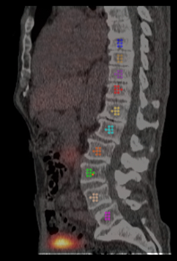
For the patients, as detailed in [6], 2-cm VOIs were manually placed in the kidneys and in up to five different dominant tumours (lesions greater than 2 cm in size, with the most prominent uptake). The bone marrow VOI was semi-automatically defined using the CT image: all voxels with Hounsfield units greater than 100 HU corresponding to L1–L4 vertebras were included.

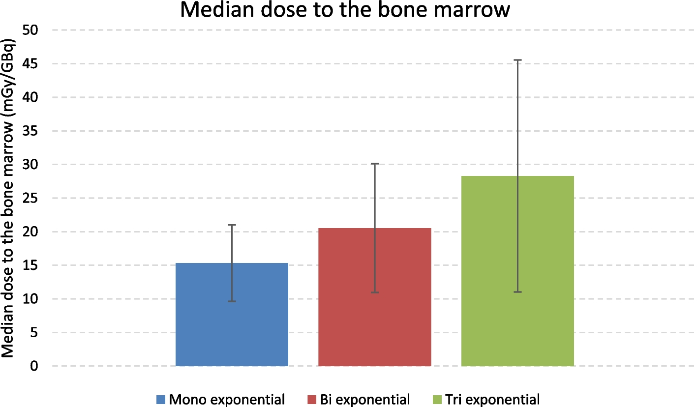
The mean counts in these VOIs were converted to activity concentration using the calibration factor and the DTCF [10]. For dosimetry, a mono-exponential curve fit was applied to the data of each VOI in addition to the averaged values for the kidneys. This allowed to determine the area under the time–activity concentration curve and to deduce the self-absorbed dose for each tissue using the activity concentration dose factor [2].

SPECT calibration

The calibration factor (CF) and dead-time constant (τ) of the Symbia have previously been determined by Frezza et al. [10]. These parameters were determined for the Intevo using the full range of quantifiable phantom data obtained. In brief, the observed wide-spectrum count rate (RWo) is expressed in relationship with the activity (A) times RWo divided by the observed primary count rate (RPo) within the phantom VOI [10]. Data points were then fitted to the following equation derived from the Sorenson’s paralysable model to resolve the calibration factor and dead-time constant using Python 3.6 (Lmfit package, least-square minimization) [8, 10, 11]:

$$R_}}} = } \cdot A \cdot \frac}}} }}}}} }} \cdot e^} \cdot A \cdot \frac}}} }}}}} }} \cdot \tau }}.$$

Once the dead-time constant is deduced, the DTCF can be determined as the ratio of the expected (RWe) on the observed wide-spectrum count rate, using the original Sorenson’s equation:

$$R_}}} = R_}}} \cdot e^}}} \cdot \tau }}$$

$$} = \frac}}} }}}}} }}.$$

Finally, a look-up table is created, with DTCFs corresponding to ascending RWo values.

Dead-time correction methods

Based on the dead-time constant, a look-up table returning a DTCF value for a given observed wide-spectrum count rate was created. Three dead-time correction methods (DTCM) were tested in the phantom and in patients:

DTCM1—pre-reconstruction, per-projection correction A DTCF was determined for each acquired projection based on the observed wide-spectrum count rate of that projection. Then, the counts of each pixel of the projection’s photopeak, upper, and lower scatter windows were multiplied by that per-projection DTCF before reconstruction. As most SPECT reconstruction software is designed to process only integer counts, it was necessary to round the multiplied counts. Rounding to the closest integer results in inaccurate total number of lost counts injected in the image (e.g. for a DTCF of 1.15, numerous low-activity pixels containing only 1, 2 or 3 counts would be corrected to 1.15, 2.30 and 3.45, respectively, and then systematically rounded down, creating a corrected counts deficit at the image level). Instead, we rounded each pixel counts to the upper integer with a probability equal to its four-digit decimal (using a Python 3.6 script). As this method is not completely deterministic, we performed this process in triplicate, followed by the reconstruction, to evaluate the effect of its randomness component. DTCM1 was considered the reference method, being in principle the most accurate.

DTCM2—pre-reconstruction, per-volume correction Same method as DTCM1, but with all projections corrected using a single DTCF derived from the average observed wide-spectrum count rate of the entire acquisition. The purpose of DTCM2 was to rule out any bias introduced by performing the per-volume correction before versus after reconstruction, as in DTCM3.

DTCM3—post-reconstruction, per-volume correction As detailed in [4,5,6] and as currently used in our clinics, the DTCF that is derived from the average observed wide-spectrum count rate of the entire acquisition is applied to voxel counts after reconstruction. In this case, there is no need to round to integers, as a float number can be applied subsequently to VOI count data, or conveniently inserted as the “Rescale Slope” parameter (i.e. DTCF multiplied by calibration factor) of the DICOM header of the reconstructed volume converted to the PT modality, enabling to display Bq/mL or standardised uptake values directly in the image viewer.

Analyses and statistics

For each VOI on the phantom and patient images, the dead-time corrected counts per second according to each DTCM were quantified with the previously determined calibration factor. For the phantom, the estimated quantified activity concentrations for each VOI were also compared with the true activity concentrations. For DTCM1 and DTCM2, the coefficient of variation among the three repetitions was computed for each VOI. The relative differences in counts (and thus in activity concentration) and absorbed doses (in patients) were compared between the DTCMs. All statistics and graphs were generated on R 4.1 (RStudio Inc., Boston, MA, USA, ggplot2 package).