2.1 Sample and Four-Wave Mixing Dynamics

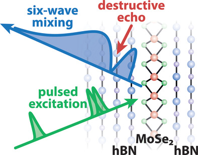
We perform multi-wave mixing experiments on an hBN/MoSe2/hBN heterostructure as schematically depicted in Figure 1. By radio frequency modulating the incoming beams, the different pulses are labeled by phases ϕj.[40] After heterodyning the emitted light with a specific N-wave mixing (NWM) phase, that is a particular phase combination of the form ϕNWM = ∑jajϕj (aj∈Z, ∑j|aj| = N − 1, ∑jaj = 1), we retrieve the corresponding nonlinear signal from the investigated monolayer.[41] Details are given in the experimental section. We use the same sample as investigated in ref. [35] where the echo formation in two-pulse FWM signals with ϕFWM = 2ϕ2 − ϕ1 was used to study the inhomogeneity of the structure. The well known photon echo appears due to the dephasing impact of the structural inhomogeneity on the exciton's coherence as schematically depicted via Bloch vectors in Figure 2.[42] For the sake of simplicity in the illustration we show a combination of a π/2 and a π pulse, which results in a photon echo in the full coherence. However, when considering the FWM coherence characterized by the phase ϕFWM the photon echo appears for any combination of pulse areas. The first laser pulse in Figure 2a having a pulse area of θ1 = π/2 and arriving at the time t = −τ generates an exciton coherence. Because of the presence of different transition energies, originating from strain and dielectric variations, the coherences generated by the first laser pulse oscillate with different frequencies resulting in a dephasing of the total coherence. As depicted in Figure 2b, after a delay τ, that is, at the time t = 0, a second laser pulse with the pulse area θ2 = π inverts all Bloch vectors. This is followed by a rephasing of the different coherences. The rephasing takes the same time as the dephasing and therefore the FWM signal is significantly enhanced due to constructive interferences at the time precisely given by the delay time t = τ between the two pulses.

Sample structure consisting of a multilayer hBN, monolayer MoSe2, multilayer hBN stack. (Left) Four-wave mixing (FWM) generated by two laser pulses with tunable delay τ. (Right) Six-wave mixing (SWM) with three excitation pulses having a tunable delay τ between pulses 2 and 3. The FWM and SWM dynamics are measured in real time t.

Schematic Bloch vector image of the photon echo process. a) 1st laser pulse excitation with following dissipation. b) 2nd excitation inverting all coherences and following rephasing. Laser pulse rotations are depicted in green, initial and final Bloch vectors in grey and blue, respectively, and the inhomogeneity induced coherence dynamics in red.

In Figure 3a we show the measured FWM signal from our sample as a function of the real time t after the second pulse and the delay τ. The pulse alignment is such that the pulse with phase ϕ1 arrives at t = −τ and the pulse with ϕ2 at t = 0. We find that the amplitude is not concentrated along the diagonal, which would represent a photon echo. Instead, starting from its maximum around (τ, t) = (0, 0) it basically decays to positive delays and times. This demonstrates that the investigated sample position is virtually homogenous because the photon echo is not present. Figure 3b shows the corresponding simulated FWM amplitude |SFWM| within a few-level system where we take the exciton transfer into the optically uncoupled valley as well as the exciton-exciton interaction in terms of the local field model into account. It describes the optically induced dynamics of the exciton's coherence p and its occupations n and n′ via[11, 43, 44]

dpdt=i(1−2n)[Ω(t)+Vp]−(β+iω0)p(1a)

dndt=2Im[Ω∗(t)p]−Γn−λ(n−n′)(1b)

dn′dt=−Γn′−λ(n′−n)(1c)

Four-wave mixing dynamics as a function of real time t and delay τ. a) Experiment and b) simulation.

Here, n and n′ are the occupations in the optically coupled and uncoupled valleys, respectively, Ω(t) is the time dependent Rabi frequency describing the optical excitation by co-circlarly polarized pulses, β and Γ are the dephasing and the decay rate, respectively, ℏω0 is the exciton energy in the absence of the local field coupling, and V is the strength of the local field coupling. Compared to ref. [44] we do not find a significant impact of excitation induced dephasing as discussed in more detail in the Supporting Information. As recently studied in ref. [44] we additionally take an intervalley scattering contribution with the rate λ into account. In the special case λ = 0, the system reduces to a two-level system. We have recently investigated the local field model in the context of nonlinear optical signals focussing on FWM[43] and pump-probe spectroscopy,[44] showing that the handy description produces resonant optical spectroscopy signals that are consistent with experiments. In a nutshell, the local field effect leads to energy shifts of the exciton depending on the its occupation. In the limit of ultrafast optical pulses Equation (1) can be solved analytically relating the coherence p+ and the occupation n+ after the pulse to the respective values p− and n− immediately before the pulse

p+=p−cos2θ2+i2sin(θ)(1−2n−)eiϕ+sin2θ2p−∗ei2ϕ≈p−+iθ2(1−2n−)eiϕ(2a)

n+=n−+sin2θ2(1−2n−)+sin(θ)Imp−e−iϕ≈n−+θImp−e−iϕ,(2b)

where θ is the pulse area and ϕ its phase. The approximations in Equation (2) describe the light-field induced contributions of a single pulse in first order of the pulse area, which is sufficient for reproducing the contributions of the order V2 to the SWM signal, discussed in the main text of this work (other contributions, involving terms up to the second order in the pulse areas, are discussed in the Supporting Information). Starting from the excitonic ground state characterized by n=n1−=0, p=p1−=0 the first pulse in the linear order creates

p1+≈iθ12eiϕ1(3a)

n1+≈0(3b)

which shows that relevant exciton occupations will only be created by a second laser pulse from p1+. Our goal is to derive the nonlinear optical response in the lowest order of the pulse area θ because the experiments are performed with low pulse powers. In the case of the SWM signal this is the fifth order O(θ5) (χ(5)-regime). Once optical pulses have generated coherences p0 and occupations n0 the corresponding free propagation [Ω = 0, in Equation (1)] is governed by pure dephasing of p, exciton decay and intervalley scattering of n(′), and local field coupling between p and n. The corresponding dynamics can also be calculated analytically. Focusing on the optically addressed occupation first, its time-dependence reads

n(t)=n0+n0′2e−Γt+n0−n0′2e−(Γ+2λ)t(4a)

which leads to a balanced occupation between the two valleys n and n′ on the timescale 1/(2λ) and a decay of both occupations with the rate Γ. As known from literature[44-46] and as considered in this work the intervalley scattering is typically significantly faster than the decay, that is, Γ ≪ 2λ. As a simplifying approximation for the sake of interpreting the results we can therefore assume that the occupations are balanced rapidly after an optical pulse, that is,

n(t)≈n0+n0′2e−Γt(4b)

This step might lead to slight deviations for short delays in the range τ ≈ 1/(2λ) which are however hardly visible for the parameters chosen here as shown in the Supporting Information. Further we can only optically manipulate the occupation n, while n′ remains unchanged by the applied laser pulses. According to Equation (3a) these pulses moreover add phase labels ϕ. As explained at the beginning of this section and as practically applied below, we are only interested in specific phase combinations that describe the considered wave-mixing signal. Consequently, any change of the occupation n is labeled by phase factors which do not apply to the other valley n′. Therefore, the latter is irrelevant for the final optical signal and we can consider n0′=0 in Equation (4b) resulting in

n(t)≈n02e−Γt(4c)

We want to remark that in the opposite limit of a very slow scattering rate 2λ ≪ Γ the occupation dynamics would directly be given by n(t) = n0e−Γt. In this case all later discussions would work in the same way. By replacing V → 2V in all the following derivations, one can even directly retrieve the corresponding equations. Based on this approximation for the occupation dynamics we can calculate the coherence dynamics in the frame rotating with ω0−V

p(t)=p0exp−i2VΓ∫t0dt′n(t′)e−iβt≈p0exp−i2VΓn021−e−Γte−iβt≈p0eiVn0te−iβt≈p01−iVn0t−12(Vn0t)2e−iβt(5)

In the first approximation step, we have used the approximated occuption from Equation (4c). As the exciton decay is much slower than the dephasing Γ ≪ β, in the second step we take Γ → 0. Finally, we keep the local field-induced contributions up to the second order in the exciton occupation, that is, considering Vn0t ≪ 1. Below we will see that these are the terms which contribute to the SWM signal in the χ(5)-regime. In the Supporting Information, we show that only terms up to O(V2) contribute to the χ(5)-regime of the SWM signal, while contributions with higher powers in V appear in higher orders of the optical field. The last equation tells us that the local field induced mixing of the occupation n0 with the coherence p0 into the coherence p(t) in the lowest order grows linearly in time with a rate given by n0 and the local field strength V. We will use this argument later on.

We simulate the FWM signal with the phase combination 2ϕ2 − ϕ1 by calculating the coherence dynamics p(t) following a two-pulse sequence and filter this quantity with respect to the required phase combination as described in refs. [43, 44]. With this we find the signal dynamics |SFWM|≈|2ϕ2−ϕ1p2(t,τ)| depicted in Figure 3b. To achieve the excellent agreement with the experiment in Figure 3a, we used a local field strength of V = 100 ps−1 and pulse areas of θ1 = θ2/2 = θ = 0.02π, a Gaussian pulse duration of Δt = 70 fs (standard deviation), a dephasing rate of β = 3 ps−1, an intervalley scattering rate λ = 4 ps−1, and a decay rate of Γ = 0.6 ps−1. Note that the depicted signal was calculated numerically because we considered a non-vanishing pulse duration and we did not employ the approximations mentioned in Equations (2)–(5). To set the strength of the local field coupling into context, typical values for GaAs quantum wells were reported in the range of a few meV,[47, 48] which is at least one order of magnitude smaller than considered here.

2.2 Six-Wave Mixing Dynamics

In the present study we go one step further in multi-wave mixing and consider one of the possible SWM signals generated by three laser pulses, namely ϕSWM = 2ϕ3 − 2ϕ2 + ϕ1. In principle there are two delays in this pulse sequence that could be varied but, as schematically shown in Figure 1 (right), we set the delay between the first two pulses to τ12 = 0 and only vary the second one τ23 = τ. The impact of a non-vanishing τ12 is discussed in the Supporting Information. In the pure two-level system this configuration probes the polarization, that is, it contains the same information as the FWM signal discussed before as shown in the Supporting Information. The measured SWM dynamics as a function of the real time t after the third pulse and the delay τ are shown in Figure 4a. Here, the two pulses with ϕ1 and ϕ2 arrive at t = −τ and the pulse with ϕ3 at t = 0. The signal consists of a strong maximum at small t ≈ 0.5 ps and τ ≈ 0. Moving to negative delays τ < 0 (pulse 3 is arriving before 1 and 2), the signal is strongly damped. For positive delays τ > 0 it decays much slower on the same timescale as the FWM signal in Figure 3. We find a remarkable depression of the signal that stretches along the curved diagonal given by Equation (9) (dashed black line), as will be derived below. In correspondence with the previously described constructive signal enhancement in the photon echo, we call this pronounced signal reduction a destructive photon echo. Later, we will discuss criteria justifying the labeling of this feature as an echo effect.

Six-wave mixing dynamics as a function of real time t and delay τ. a) Experiment, b) simulation, with the curved dashed line depicting Equation (9).

To identify the origin of this peculiar dynamical feature we model the SWM signal within the local field model described above. We consider the same system parameters as for the FWM signal but choose equal pulse areas for all three pulses θ1 = θ2 = θ3 = θ = 0.02π, in agreement with the experiment. In the Supporting Information, it is shown that the exact choice of θ in the low excitation regime does not change the SWM signal dynamics. The SWM signal is extracted via the phase combination 2ϕ3 − 2ϕ2 + ϕ1 and the signal dynamics |SSWM|≈|2ϕ3−2ϕ2+ϕ1p3(t,τ)| are depicted in Figure 4b. The retrieved signal agrees very well with the respective experiment in Figure 4a showing the same characteristic suppression of the signal, that is, the destructive photon echo. We give an overview regarding the impact of the different parameters on the SWM signal in the Supporting Information. Most importantly, it is shown in the Supporting Information, that the SWM dynamics do not exhibit the suppression for small local field strengths V demonstrating that this feature is a result of exciton-exciton interaction. Other specific features in the signal's dynamics like the asymmetric decay between positive and negative delays or between τ and t were studied in detail in ref. [43] and behave similarly in SWM. The destructive photon echo effect should also be present in an inhomogeneously broadened system, where also a traditional constructive photon echo develops. As the constructive echo selects only a specific time interval of the emitted signal around t = τ, it leads to a suppression of the entire SWM signal for all other times. Consequently, the SWM signal and therefore the destructive photon echo, which bends away from the diagonal (discussed later), are only visible in the vicinity of t = τ. This aspect is studied in more detail in the Supporting Information.

Note, that the simulation shown in Figure 4b takes the non-vanishing pulse duration into account and is therefore performed numerically. In the limit of ultrafast laser pulses we can find analytical expressions for the SWM signal. Given that the experiment is carried out with weak pulse powers, we restrict the following studies on the lowest order in the optical field which is the χ(5)-regime. In this order we have already eight different contributions as derived in the Supporting Information. From these we will focus on the ones with the strongest local field contribution which is O(V2), that is, we omit all terms O(V1) and O(V0). The reason for this is the absence of the destructive echo for small V. In ref. [43] we have derived a flow chart representation for the construction of nonlinear wave mixing signals. In Figure 5 we employ this procedure to disentangle the origin of the different contributions to the SWM signal. The flow chart only shows coherences p (blue) and occupations n (red) with phase combinations (green, given as left indices) relevant for the final signal; corresponding flow charts for the contributions with O(V1) and O(V0) are provided in the Supporting Information. Conveniently, the O(V2)-contributions can be derived with the approximations given in Equation (2). Note, that we introduce phase differences Δnm = ϕn − ϕm here. The right lower index refers to the pulse number, while the upper − (+) indicates times immediately before (after) that pulse. Starting from the excitonic ground state with n = 0, p = 0 the first pulse generates the occupation 0n1+ and the coherence ϕ1p1+. Note, that in the scheme we do not restrict ourselves to the lowest order contributions in the light field and thus include also the occupation which is of second order in the pulse amplitude. The second pulse arrives at the same time (τ12 = 0) and creates two occupations 0n2+ and |Δ21|n2+ and the coherence ϕ2p2+. During the following propagation for the time of the delay τ two relevant things happen: On the one hand all coherences experience dephasing (blue arrows). On the other hand ϕ2p2+ is mixed with |Δ21|n2+ via the local field coupling resulting in the coherence 2ϕ2−ϕ1p3− before the third pulse. Note, that this contribution carries the FWM phase ϕFWM = 2ϕ2 − ϕ1 which we will come back to below. After the final third pulse we have five relevant terms[49]: The coherence ϕ3p3+ and the three occupations |Δ32|n3+, |Δ32−Δ21|n3+, and |Δ21|n3+. The polarization ϕ1p1+ is not affected by the second and third pulse and just evolves into ϕ1p3+. During the remaining propagation step in real time t the three relevant SWM contributions are generated by local field mixing processes according to Equation (5).

Flow chart for the three main contributions to the SWM signal listing intermediate phase-filtered coherences (p, blue) and occupations (n, red). Green waved arrows show pulse induced, violet dotted ones local field induced, black ones free dynamics without, and blue ones with dephasing. The phase differences are defined as Δnm = ϕn − ϕm. The flow chart holds for any order of the optical field. However, in the linear response regime considered here, it is 0n1+=0n2+=0n3−=0.

Considering the contribution on the right first, we have to mix ϕ1p3+ with |Δ32|n3+ twice. This results in the phase combination ϕ1 + 2(ϕ3 − ϕ2) which is the SWM phase combination. According to Equation (5), each of these local field mixing processes contributes with an amplitude of Vt resulting in the amplitude (Vt)2. In addition the amplitude is damped due to the dephasing happening during the delay. Following the two paths in the diagram back to this propagation step we find that ϕ1p2+→ϕ1p3− and ϕ2p2+→ϕ2p3− contribute with a dephasing term ∼e−βτ. The latter one is used twice due to the double local field mixing resulting in the total damping rate of e−3βτ.

Moving on to the left contribution in Figure 5, we find that in the last propagation the coherence ϕ3p3+ is local-field mixed with |Δ32|n3+ and |Δ21|n3+ once, resulting in the SWM phase combination ϕ3 + (ϕ3 − ϕ2) − (ϕ2 − ϕ1). Each of these processes contributes an amplitude of Vt again resulting in (Vt)2. The difference to the first term is that here only |Δ32|n3+ stems from a coherence, namely ϕ2p2+ which experiences a dephasing during the delay. Consequently, the entire contribution is damped by e−βτ. This already shows that this contribution is more important for the final SWM signal than the right term discussed first.

The final main contribution is the middle one in Figure 5. Here, in the last real time propagation the local field mixing happens between ϕ3p3+ and |Δ32−Δ21|n3+ which contributes with an amplitude of Vt. Following the path back, we find that the occupation is created from the polarization 2ϕ2−ϕ1p3− which itself is produced by a local field mixing step between ϕ2p2+ and |Δ21|n2+. The mixing process lasts for the delay time and therefore contributes with a factor Vτ to the final SWM amplitude. This is also the step where the only dephasing happens resulting in a final amplitude of V2τte−βτ.

Directly comparing the three contributions in Figure 5 we find that the right one is smaller than the other two due to the stronger dephasing during the delay. We will therefore disregard this term from now on. The other two terms are of the order V2 and exhibit the same dephasing with e−βτ. From the full derivation given in the Supporting Information we find that these two terms in Figure 5 carry opposite signs. We will explain these signs later when introducing an effective Bloch vector picture to illustrate the destructive echo formation. Finally, adding the two terms we get

SWMp3(t,τ)∼V2(τt−t2)e−β(τ+t)(6)

where we also added the dephasing rate for the propagation in t after the last pulse. We find that the two terms exactly compensate each other for t = τ. This renders our first step toward the understanding of the destructive echo. We identified two paths (signal contributions) with the same damping but with different magnitudes depending on the delay τ that act destructively in the total SWM signal. To illustrate the interplay between these two terms in Figure 6 we schematically plot the applied laser pulses and the absolute value of the final SWM signal retrieved from the previous derivations. We also include the intermediate growth of the FWM coherence lasting for the delay τ.

Schematic picture of the pulse sequence and signal development from the two main contributions.

The full SWM signal in the χ(5)-regime is derived in the Supporting Information and reads

SWMp3(t,τ)=θ25i+V(τ−4t)−i2(Vt)2e−2βτ+iV2t(τ−t)e−β(t+τ)(7)

Interestingly, we also find a suppression of the signal when only considering the terms O(V1), namely for t = τ/4. We obviously do not find such a feature in our measurement, which shows that the linear order in V does not have a significant contribution.

One advantage of the spectral interferometry in the applied approach is the possibility to detect—besides the amplitude—also the phase of the SWM signal.[50] We see that for t < τ the positive contribution ∼τt dominates while for t > τ the negative one ∼−t2 is larger. Therefore we expect a phase jump when crossing the destructive echo in time t < τ → t > τ. To confirm this in Figure 7a, we plot the measured (solid blue) and calculated (dashed red) SWM signal amplitude as a function of time t for τ = 0.35 ps. We slightly adjusted the pulse duration to Δt = 80 fs to achieve the good agreement with this experiment. The finding that the simulated signal does not drop to zero shows the impact of the non-compensating con