
記住我


Spatial navigation requires active exploration, multisensory integration, as well as the encoding and long-term consolidation of internal models of the world (Arleo & Rondi-Reig, 2007; Epstein et al., 2017; Wolbers & Hegarty, 2010). Thus, the ability to navigate in space encompasses both perceptual and cognitive faculties (Ekstrom et al., 2017; Spiers & Barry, 2015). A large body of work has elucidated the neural bases of wayfinding behavior in both animals and humans, leading to a better understanding of the navigational system across multiple levels (Burgess, 2008; Epstein et al., 2017; Hardcastle et al., 2017; Poulter et al., 2018).
Most investigations of the brain network subtending human spatial navigation rely on functional magnetic resonance imaging (fMRI) (Epstein et al., 2017; Taube et al., 2013) due to its unmatched spatial resolution among non-invasive methods. However, this technique is not suited for testing participants in unconstrained motion conditions, which limits the study of neural processes involved during natural behavior (Zaitsev et al., 2015). Combining behaviometric and neurometric recordings in ecological (i.e., close to real, natural) conditions is key to modern cognitive neuroscience (Ladouce et al., 2019; Schaefer, 2014), in particular to study spatial cognition (Bécu et al., 2020a; Gehrke & Gramann, 2021; Miyakoshi et al., 2021). With relatively coarse spatial but fine temporal resolution, electroencephalography (EEG) offers a complementary tool for neuroimaging the brain during spatial behavior (Baker & Holroyd, 2009; Bischof & Boulanger, 2003; Lin et al., 2009, 2015; Plank et al., 2010). Although EEG does not prevent the participant's motion per se, it is very sensitive to movement-related artifacts. Electrical potentials from muscle contractions (e.g., head movements, eye blinks, or heartbeat, see Jung et al., 2000) generate strong artifactual signals that compromise the extraction of brain-related responses (i.e., reducing the signal-to-noise ratio). As a consequence, most EEG studies have constrained the mobility of participants in order to minimize motion-related artifacts (e.g., by making them sit in front of a screen and respond with finger taps only).
Recent technical developments have unlocked the possibility of using EEG brain imaging in a variety of ecological conditions (indoor walking: Luu et al., 2017a; Ladouce et al., 2019; Park & Donaldson, 2019; outdoor walking: Debener et al., 2012; Reiser et al., 2019; cycling: Zink et al., 2016; di Fronso et al., 2019; and dual tasking: Marcar et al., 2014; Bohle et al., 2019). By coupling EEG recordings with other biometric measures (e.g., body and eye movements), the Mobile Brain/Body Imaging (MoBI) approach gives access to unprecedented behavioral and neural data analysis (Gramann et al., 2011, 2014; Ladouce et al., 2017; Makeig et al., 2009). In addition, the MoBI paradigm has been successfully combined with fully immersive virtual reality (VR) protocols (Djebbara et al., 2019; Liang et al., 2018; Peterson & Ferris, 2019; Plank et al., 2015; Snider et al., 2013). Immersive VR allows near-naturalistic conditions to be reproduced, while controlling all environmental parameters (Diersch & Wolbers, 2019; Park et al., 2018; Parsons, 2015; Starrett & Ekstrom, 2018). The reliability of 3D-immersive VR enables the stimulation of visual, auditory, and proprioceptive modalities, while allowing the participant to actively explore and sense the virtual environment (Bohil et al., 2011; Kober et al., 2012). This continuous interplay between locomotion and multisensory perception is thought to be a key component of spatial cognition in near-natural conditions, as its absence leads to impaired performance in various spatial abilities (path integration: Chance et al., 1998; spatial updating: Klier & Angelaki, 2008; spatial reference frame computation: Gramann, 2013; spatial navigation and orientation: Taube et al., 2013; Ladouce et al., 2017; and spatial memory: Holmes et al., 2018).
In the present study, we use the MoBI approach to combine high-density mobile EEG recordings and immersive VR in order to study spatial navigation in a three-arm maze (i.e., a Y-maze). Our primary aim is to provide a proof-of-concept in terms of EEG-grounded neural substrates of landmark-based navigation consistent with those found in similar fMRI paradigms (Iaria et al., 2003; Konishi et al., 2013; Wolbers & Büchel, 2005; Wolbers et al., 2004). We chose the Y-maze task because it offers a simple two-choice behavioral paradigm suitable to study landmark-based spatial navigation and to discriminate between allocentric (i.e., world-centered) and egocentric (i.e., self-centered) responses, as previously shown in animals (Barnes et al., 1980) and humans (Bécu et al., 2020b; Rodgers et al., 2012). Complementarily, a recent fMRI study of ours has investigated the brain activity of regions involved in visuo-spatial processing and navigation in a similar Y-maze task (Ramanoël et al., 2020). This offers the opportunity to comparatively validate the neural correlates emerged through static fMRI experiment against those found by mobile high-density EEG.
The neural substrates of landmark-based navigation form a network spanning medial temporal areas (e.g., hippocampus and para-hippocampal cortex) and medial parietal regions (Epstein & Vass, 2014), such as the functionally defined retrosplenial complex (RSC) (Epstein, 2008). Here, we expect the RSC to play a role in mediating spatial orientation through the encoding and retrieval of visual landmarks (Auger & Maguire, 2018; Auger et al., 2012, 2015; Julian et al., 2018; Marchette et al., 2015; Spiers & Maguire, 2006). The RSC is indeed implicated in the translation between landmark-based representations in both egocentric and allocentric reference frames (Marchette et al., 2014; Mitchell et al., 2018; Shine et al., 2016; Sulpizio et al., 2013; Vann et al., 2009). Our hypothesis also encompasses the role of specific upstream, visual processing areas of the parieto-occipital region involved in active wayfinding behavior (Bonner & Epstein, 2017; Patai & Spiers, 2017). In addition, our paradigm accounts for the role of downstream, higher-order cognitive functions necessary for path evaluation, covering a frontoparietal network (including prefrontal areas, Epstein et al., 2017; Spiers & Gilbert, 2015) that codes for overarching mechanisms such as spatial attention and spatial working memory (Cona & Scarpazza, 2019).
Mobile brain imaging protocols also engage locomotion control processes, in which motor areas in the frontal lobe and somatosensory areas in the parietal lobe are typically involved (Gwin et al., 2010; Seeber et al., 2014; Roeder et al., 2018; see Delval et al., 2020 for a recent review). Furthermore, the integration of vestibular and proprioceptive cues made possible by mobile EEG paradigms is likely to influence the observed neural correlates of spatial orientation (Ehinger et al., 2014; Gramann et al., 2018) and attention (Ladouce et al., 2019).
Finally, given the high temporal resolution of EEG, we aim at characterizing how the activity of the structures engaged in active, multimodal landmark-based navigation is modulated by behavioral events, related to either action planning (e.g., observation of the environment, physical rotation to complement mental perspective taking) or action execution (e.g., walking, maintaining balance). We also aim at exploring the differential engagement of brain regions involved in the encoding (learning condition) and the retrieval (control and probe conditions) phases of the task (RSC is implicated in both; Burles et al., 2018; Epstein & Vass, 2014; Mitchell et al., 2018).
The purpose of this study is thus to explore the cortical correlates of landmark-based navigation in mobile participants. We first hypothesize that the analysis of the EEG signal will retrieve the above-mentioned brain structures known to be engaged during active spatial navigation based on visual cues. We then expect behavioral events to modulate features of the recorded EEG data, identifiable as transient time–frequency patterns in the involved brain areas, and to interpret them with respect to spatial cognition and locomotion control literature. Finally, we expect to find significant differences in these patterns across the phases of the task, contrasting the cognitive mechanisms involved in context-dependent task solving. We aim to investigate and interpret their condition specificity and their temporality. Under such considerations, this work can help toward a better understanding of context-specific neural signatures of landmark-based navigation.
2 METHODS 2.1 ParticipantsSeventeen healthy adults (range: 21–35 years old, M = 26,82, SD = 4,85; 10 women) participated to this study. Fifteen were right-handed and two left-handed. All participants had normal (or corrected to normal) vision and no history of neurological disease. In one recording session, there were abnormalities (discontinuities and absence of events) in the motion capture signal. Thus, we removed one participant from the analysis. The experimental procedures were approved by the local ethics committee (GR_12_20190513, Institute of Psychology & Ergonomics, Technische Universität Berlin, Germany) and all participants signed a written informed consent, in accordance with the Declaration of Helsinki. All participants answered a discomfort questionnaire at the end of the experiment, adapted from the simulation sickness questionnaire of Kennedy et al. (1993), which can be found in Methods S1. We gave the instructions in English and all participants reported a good understanding of the English language. Each participant received a compensation of either 10€/h or course credits.
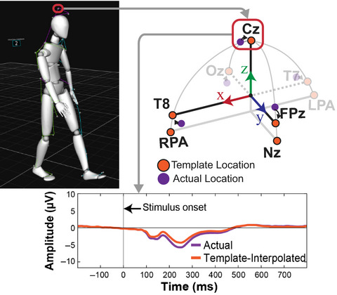
2.2 EEG systemThe EEG system (Figure 1a) consisted of 128 active wet electrodes (actiCAP slim, Brain Products, Gilching, Germany) mounted on an elastic cap with an equidistant layout (EASYCAP, Herrsching, Germany). The impedance of a majority of the channels was below 25 kΩ (9.5% of the electrodes had an impedance above 25 kΩ). Two electrodes placed below the participant's eyes recorded electro-oculograms (EOG). An additional electrode located closest to the standard position F3 (10–20 international system) provided the reference for all other electrodes. The EEG recordings occurred at a sampling rate of 1 kHz. The raw EEG signal was streamed wirelessly (BrainAmp Move System, Brain Products, Gilching, Germany) and it was recorded continuously for the entire duration of the experiment.

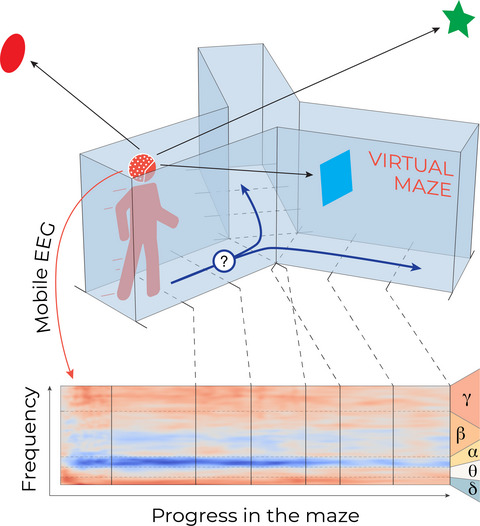
Virtual environment, setup, and timeline of the experiment. (a) Details of participant's equipment. (1) EEG cap (128 channels); (2) VR Head-mounted display (VIVE Pro); (3) Wifi transmitter for EEG data (Move system); (4) Additional motion capture tracker (VIVE tracker); and (5) Backpack computer running the virtual environment (Zotac PC). (b) Virtual environment. Participants explored a virtual equilateral Y-maze. In the learning condition, they always started in the same arm (e.g., A) and they had to find a hidden goal, always placed in the same location (e.g., C). In the testing conditions, the environment and goal location stayed the same but the participant would start from either the same position (A) in control trials or the third arm (B) in probe trials. (c) Spatial discretization of the environment (example for a learning trial). We delimited 10 areas in the maze: “S” stands for starting arm, “C” for center, “E” for error arm, and “G” for goal arm. In the text, when referring to the arm chosen by the participant (either “E” or “G”), we use the letter “F” standing for finish arm. These labels are condition-dependent (different in the probe condition). The names of the landmark depend on the location of starting arm in the learning condition and goal arm. These names are block dependent. (d) General timeline of the experiment. The first row represents the general succession of conditions in the experiment. The second row shows an example of the sequence of trials in an experimental block. The third row illustrates the structure of a trial, including a possible course of events: progress across spatial sections and visibility of landmarks depending on participant's head movements. We provide a video of a participant performing the task, along with the reconstruction of the tracker positions, in Video S1
2.3 Virtual Y-maze and motion trackingThe virtual maze consisted of an equilateral Y-maze (3-armed maze) with three distal landmarks placed outside the maze, 20 m away from the center and visible above the walls (Figure 1b). The landmarks were abstract geometric shapes (e.g., square, circle, star). The wall texture and the light were homogeneous and non-informative. Each arm of the maze was 90 cm wide and 225 cm long. For the sake of analysis, the maze was discretized into 10 zones (3 evenly divided zones per arm and one for the maze center, Figure 1c). These zones were not visible to the participant. Crossing between zones was recorded online without influencing the task flow.
We designed the virtual Y-maze by using the Unity3D game engine (Unity Technologies, San Francisco, California, USA, version 2017.1.1f1 for Windows), and we rendered it using an HTC Vive Pro head-mounted display (HTC Corporation, Taoyuan, Taïwan) with a 90 Hz refresh rate (2 times AMOLED 3.5” 1440x1600 pixels, 615 ppi, and 110° nominal field of view). The HTC was connected to a VR capable backpack computer (Zotac PC, Intel 7th Gen Kaby Lake processor, GeForce GTX 1060 graphics, 32GB DDR4-2400 memory support, Windows 10 OS, ZOTAC Technology Limited, Fo Tan, Hong Kong) running on batteries and controlled remotely (Figure 1a). An integrated HTC Lighthouse motion tracking system (four cameras, 90 Hz sampling rate, covering an 8 × 12 m area) enabled the recording of the participant's head by tracking the HTC Vive Pro head-mounted display. It also enabled the tracking of the torso movements via an additional HTC Vive Tracker placed on the participant's backpack. We virtually translated the position of this tracker to better reflect the real position of the participant's torso by considering his or her body measurements. The torso tracker was also used to trigger spatial events (e.g., reaching the goal, crossing spatial section boundaries). The height of the maze walls and the altitude of landmarks were adjusted to the participant's height (based on the head tracker) to provide each participant with the same visual experience. Each participant wore earphones playing a continuous white noise to avoid auditory cues from the external world. During the disorientation periods (see protocol), relaxing music replaced the white noise. One experimenter gave instructions through the earphones, while monitoring the experiment from a control room. The participant could answer through an integrated microphone. He/she was instructed to refrain from talking while performing the experiment to limit artifacts in the recorded EEG signal. Another experimenter stayed with the participant inside the experimental room to help with potential technical issues and conduct the disorientation, avoiding any interaction with participants during the task. The EEG signal, motion capture, and all trigger events were recorded and synchronized using the Lab Streaming Layer software (Kothe, 2014).
2.4 Experimental protocolAn entire experimental session lasted 3 hr on average and it included preparing the participant with the EEG and VR equipment and running the experimental protocol. The immersion time in VR was between 60 and 90 min.
2.4.1 Free exploration phaseBefore starting the actual task, the participant explored the Y-maze for 3 min, starting at the center of the maze. He/she was instructed to inspect all details of the environment and to keep walking until the time elapsed. The purpose of this phase was to familiarize the participant to the VR system and the Y-maze environment (including the constellation of landmarks).
2.4.2 Navigation taskThe navigation task included a learning condition and a testing condition. During learning, the participant began each trial from the starting arm (e.g., location A in Figure 1b) and he/she had to find the direct route to a hidden target at the end of the goal arm (e.g., location C in Figure 1b). Upon reaching the goal, a reward materialized in front of the participant (3D object on a small pillar representing, for instance, a treasure chest) to indicate the correct location and the end of the current trial. The learning period lasted until the participant reached the goal directly, without entering the other arm, three times in a row. Before each trial, we disoriented the participant to ensure that he/she would not rely on previous trials or the physical world to retrieve his/her position and orientation. To disorient the participant, the experimenter simply walked him/her around for a few seconds with both eyes closed (and the head-mounted display showing a black screen). The testing condition included six trials: three control trials and three probe trials, ordered pseudo-randomly (always starting with a control, but never with three control trials in a row). In the control trials, the participant started from the same arm as in the learning condition (e.g., location A in Figure 1b). In the probe trials, he/she started from the third arm (e.g., location B in Figure 1b). Before starting a new trial (either control or probe), the participant was always disoriented. Then, he/she had to navigate to the arm where he/she expected to find the goal and stop there (without receiving any reward signal). If the participant went to the incorrect arm, it was considered as an error. We present a single trial example of one participant performing the task and we illustrate the motion tracking in the virtual environment in Video S1.
2.4.3 Block repetitionsThe sequence “learning condition + testing condition” formed an experimental block. Each participant performed nine experimental blocks (Figure 1d). In order to foster a feeling of novelty across block repetitions, we varied several environmental properties at the beginning of each block: wall texture (e.g., brick, wood, etc.), goal location (i.e., in the right or left arm, relative to the starting arm), reward type (e.g., treasure chest, presents, etc.), as well as the shape (e.g., circle, square, triangle, etc.) and color of landmarks. When changing the environment between blocks, we kept the maze layout and landmark locations identical. The sequence of blocks was identical for all participants, who had to take a compulsory break after the fourth block (Figure 1d). In addition, after the sixth or seventh block, a break was introduced when requested by the participant.
2.4.4 EEG baseline recordingsBoth before the free exploration period and after the 9th block, the participant had to stand for 3 min with his/her eyes opened in a dark environment. This served to constitute a general baseline for brain activity. Similarly, we recorded the EEG baseline signal (in the dark for a random duration of 2–4 s) before each trial (Figure 1d, bottom). Besides providing a baseline EEG activity specific to each trial, this also allowed the starting trial time (i.e., the appearance time of the maze) to be randomized, thus avoiding any anticipation by the participant.
2.5 Behavioral analysisAll analyses were done with MATLAB (R2017a and R2019a; The MathWorks Inc., Natick, MA, USA), using custom scripts based on the EEGLAB toolbox version 14.1.0b (Delorme & Makeig, 2004), the MoBILAB (Ojeda et al., 2014) open source toolbox, and the BeMoBIL pipeline (Klug et al., 2018).
2.5.1 Motion capture processingA set of MoBILAB's adapted functions enabled the preprocessing of motion capture data. The rigid body measurements from each tracker consisted of (x, y, z) triplets for the position and quaternion quadruplets for the orientation. After the application of a 6 Hz zero-lag low-pass finite impulse response filter, we computed the first time derivative for position of the torso tracker for walking speed extraction and we transformed the orientation data into axis/angle representations. An EEGLAB dataset allowed all preprocessed, synchronized data to be collected, and split into different streams (EEG, Motion Capture) to facilitate EEG-specific analysis based on motion markers.
2.5.2 Allocentric and egocentric groupsProbe trials served to distinguish between allocentric and egocentric responses by making the participants start from a different arm than the one used in the learning period. We assigned a participant to the allocentric group if he/she reached the goal location in the majority of probe trials (i.e., presumably, by using the landmark array to self-localize and plan his/her trajectory). Conversely, we assigned a participant to the egocentric group when he/she reached the error arm in the majority of probe trials (i.e., by merely repeating the right- or left-turn as memorized during the learning period).
2.5.3 Time to goalWe assessed the efficacy of the navigation behavior by measuring the “time to goal”, defined as the time required for the participant to finish a trial (equivalent to the “escape latency” in a Morris Water Maze). In learning trials, it corresponded to the time to reach the goal zone and trigger the reward. In test trials, it corresponded to the time to reach the believed goal location in the chosen arm (i.e., entering the G1 or E1 zone in Figure 1c).
2.5.4 Horizontal head rotations (relative heading)The participant's heading was taken as the angle formed by his/her head orientation in the horizontal plane with respect to its torso orientation, aligned with the participant's sagittal plane. After extracting the head and torso forward vectors from each tracker, computing the signed angle between those vectors' projections in the horizontal plane provided the heading value.
2.5.5 Walking speedThe forward velocity component of the torso tracker provided the participant's walking information. For each trial, we computed the mean and SD of the forward velocity, and their average for each participant. To evaluate movement onsets and offsets, we compared motion data recorded during the trials against those recorded during the short baseline period before each trial, considered as a reliable resting state for movements. Movement transitions (onsets and offsets) were based on a participant-specific threshold, equal to the resting-state mean plus 3 times the resting-state SD. The excluded movement periods were those lasting less than 250 ms and during which motion did not reach another participant-specific threshold, equal to the resting-state mean plus 5 times the resting-state SD.
2.5.6 Landmark visibilityFor analysis purposes, we named the three landmarks as Landmark 1, Landmark 2, and Landmark 3 (Figure 1c) and we tracked their visibility within the displayed scene. The participant had a horizontal field of view of 110° and a vertical field of view of 60°. Whenever a landmark appeared in the viewing frustum 1 (i.e., in the region of virtual space displayed on the screen) and it was not occluded by any wall, it was considered as visible by the participant. Given the restrained horizontal field of view and the configuration of the VR environment, perceiving more than one landmark at the same time was unlikely.
2.5.7 Zone-based behavioral analysisThe maze discretization (Figure 1c) provided a coherent basis for analyses across trials and participants. To ensure consistency in the comparison between trials, we selected those trials where the participant followed a straightforward pattern (zone-crossing sequence: S1 → S2 → S3 → C → G3 → G2 → G1). We thus discarded all trials in which the participant went backward while navigating (e.g., during learning, when his/her first choice was toward the error arm, and he/she had to come back to the center in order to go toward the goal arm). To further ensure homogeneity, we also excluded those trials in which the time to goal was unusually long (i.e., by computing the outliers of the time to goal distribution across all participants). These selection criteria kept 1,289 (of a total of 1,394) trials for analysis (see Table S1 for details about the distribution of trials across participants). Finally, we computed offline an additional event corresponding to the first walking onset of the participant in S1 (see Walking speed paragraph above for movement detection) which was inserted in the delimiting sequence of zone-crossing events. For the sake of simplicity, we used the notations “staticS1” for the period preceding this event, and “mobileS1” for the one that follows, before the participant enters S2. Hence, the complete sequence for each trial was, e.g., staticS1 → mobileS1 → S2 → S3 → C → G3 → G2 → G1.
2.5.8 Motion capture statisticsThe above zone-based discretization framed the analysis of the motion capture metrics mentioned above: walking speed, standard deviation of horizontal head rotations, and landmark visibility. For each trial, we first averaged the value of each motion variable over the period between two events of the zone sequence. Then, for each participant, we averaged these values across trials of the same condition.
To better characterize the participants' behavior in the maze, we investigated how these metrics would depend on the condition, the spatial zone, the landmark (for landmark visibility only), and the different combinations of those factors. Concerning walking speed and standard deviation of horizontal head rotations, we tested the hypothesis that participants would walk slower and make larger head movements in specific zones of the maze related to the challenge posed by the experimental condition (e.g., taking information in S1 during Learning and stopping in C to look at the constellation during Probe). Concerning landmark visibility, we tested the hypothesis that participants would make a differential use of the three landmarks (i.e., preference for one or two) and that attendance to a landmark would depend on the condition and the location of the participant in the maze (e.g., realignment with a preferred landmark at the center specific to Probe condition). We used fixed model between factors analyses of variance (ANOVAs; balanced design) to assess differences and interactions between conditions, zones, and landmarks in those dependent variables. Specifically, for the landmark visibility, we used a three-way ANOVA with the factors: condition (Learning, Control, Probe), landmark (Landmark 1, Landmark 2, Landmark 3), and zone (e.g., staticS1, mobileS1, S2, S3, Center, F3, F2). Note that “F,” standing here for “finish” arm, can be either G for “goal” or E for “error” as used in Figure 1c, depending on the trial outcome. For the walking speed and the standard deviation of horizontal head rotations, we used a two-way ANOVA with the factors condition and zone. The alpha level for significance was set at 0.01 (more conservative level taking into account that we are computing three simultaneous ANOVAs on the same dataset). When a significant main effect or interaction was found, we used pairwise t-tests (with Tukey's honest significant difference criterion method for multiple comparison correction) to unravel individual differences between factor or interaction terms.
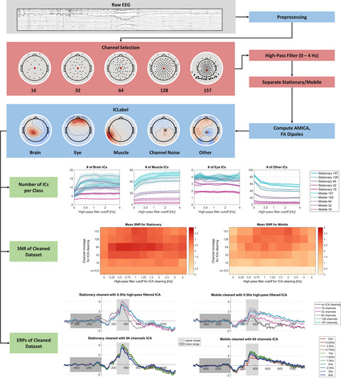
2.6 EEG data analysis overviewFigure 2 shows the outline of the data preprocessing and analysis steps.

Flowchart of the EEG processing pipeline. We first preprocessed EEG data at the individual level (in blue) and, in particular, decomposed the channel data into independent components (ICs) with an adaptative mixture ICA (AMICA) algorithm. We then selected 70 ICs per participant for the clustering procedure (in orange). Finally, we labeled and selected the clusters of interest for an ERSP analysis per condition (in brown). The “Cluster selection” process is described in the “EEG cluster analysis” section of the Results
2.7 Individual EEG analysis 2.7.1 ProcessingWe used the BeMoBIL pipeline to preprocess and clean the EEG data (Klug et al., 2018). This pipeline is fully automated and designed to improve signal-to-noise ratio (SNR) in large-scale mobile EEG datasets, which ensures full replicability of the procedure. We first downsampled the data to 250 Hz, applied a 1 Hz high-pass filter to suppress slow drifts in EEG data (zero-phase Hamming windowed finite impulse response filter with 0.5 Hz cut-off frequency and 1 Hz transition bandwidth), and removed spectral peaks at 50 Hz and 90 Hz, corresponding to power line frequency and VIVE headset refreshing rate, respectively (implemented by the cleanLineNoise function from the PREP pipeline, Bigdely-Shamlo et al., 2015). We identified noisy channels with automated rejection functions, setting parameters numerical values according to default recommendations from Bigdely-Shamlo et al. (2015). We then reconstructed the removed channels by spherical interpolation of neighboring channels and applied re-referencing to the common average. In a subsequent time-domain cleaning, we detected and removed segments with noisy data. We present more details on the implementation of the cleaning steps in Methods S2.
On the cleaned dataset, we performed an independent component analysis (ICA) using an adaptive mixture independent component analysis (AMICA) algorithm (Palmer et al., 2008), preceded by a principal component analysis reduction to the remaining rank of the dataset taking into account the number of channels interpolated and the re-referencing to the common average. For each independent component (IC), we computed an equivalent current dipole model (ECD) with the DIPFIT plugin for EEGLAB (version 3.0) (Oostenveld & Oostendorp, 2002). For this purpose, we used a common electrode location file obtained from the average of previous measures on participants wearing the same cap. We co-registered this file with a boundary element head model based on the MNI brain (Montreal Neurological Institute, MNI, Montreal, QC, Canada) to estimate dipole location. In this article, the spatial origin of an IC is approximated with the location of its associated dipole.
We opted for the BeMoBIL pipeline after comparing it against the APP pipeline (da Cruz et al., 2018), which proved to be less robust for our dataset. We based this conclusion on different metrics, by evaluating each artifactual detection step (number of channels removed, proportion of time samples excluded) and by assessing the performance of the subsequent ICA (mutual information reduction and remaining pairwise mutual information, Delorme et al., 2012). In particular, the BeMoBIL pipeline proved to be more stable and conservative than the APP pipeline (rejecting more artifactual channels and noisy temporal segments, both more consistently across participants). We detail the comparison and its results in Methods S3 and Figure S4, respectively.
2.7.2 Individual IC labelingWe used the ICLabel algorithm (version 1.1, Pion-Tonachini et al., 2019) with the “default” option to give an automatic class prediction for each IC. The model supporting this algorithm considers seven classes: (1) Brain, (2) Muscle, (3) Eye, (4) Heart, (5) Line Noise, (6) Channel Noise, and (7) Other. The prediction takes the form of a compositional label: a percentage vector expressing the likelihood of the IC to belong to each of the considered classes. Then, it compares each percentage to a class-specific threshold to form the IC label. We used the threshold vector reported by Pion-Tonachini et al. (2019) for optimizing the testing accuracy. Considering the recentness of this algorithm and the fact it has never been validated on mobile EEG data, we refined the labeling process to increase its conservativeness on Brain ICs. After the initial categorization by the algorithm, we automatically examined the ECD of ICs passing the Brain threshold and we rejected all ICs whose ECD was either located outside brain volume or exhibiting residual variance over 15% (commonly accepted threshold for dipolarity, see Delorme et al., 2012) and we put them in the “Other” class. Residual variance quantifies the quality of the fit between the actual topographic activation map and the estimated dipole projection on the scalp. Among the remaining ones, we distinguished two cases: (1) if the IC label was uniquely “Brain”, we automatically accepted it; (2) if the IC label was hybrid (multiple classes above threshold), we manually inspected the IC properties to assign the label ourselves according to the ICLabel guidelines (https://labeling.ucsd.edu/tutorial/labels – an example can be found in Figure S3). To all ICs below brain threshold, we assigned unique labels based on their highest percentage class.
2.8 Group-level EEG analysisIn order to retain maximal information for further processing, for each participant we copied the ICA results (decomposition weights, dipole locations, and labels) back to the continuous version of the dataset (i.e., the dataset before time domain cleaning in the BeMoBIL pipeline). We first band-pass filtered the data between 1 Hz (zero-phase Hamming windowed finite impulse response high-pass filter with 0.5 Hz cut-off frequency and 1 Hz transition bandwidth) and 40 Hz (zero-phase Hamming windowed finite impulse response low-pass filter with 45 Hz cut-off frequency and 10 Hz transition bandwidth). We then epoched each dataset into trials, starting at the beginning of the baseline period and ending at the time of trial completion. For each IC and each trial, we computed the trial spectrum using the pwelch method (1s Hamming windows with 50% overlap for power spectral density estimation). We baselined the spectrum with the average IC spectrum over all baseline periods using a gain model.
We additionally computed single-trial spectrograms using the newtimef function of EEGLAB (1 to 40 Hz in linear scale, using a wavelet transformation with three cycles for the lowest frequency and a linear increase with frequency of 0.5 cycles). Using a gain model, we individually normalized each trial with its average over time (Grandchamp & Delorme, 2011). Separately for each participant, we calculated a common baseline from the average of trial baseline periods (condition specific) and we subsequently corrected each trial with the baseline corresponding to its experimental condition (gain model). At the end, power data were log-transformed and expressed in decibels. To enable trial comparability, these event-related spectral perturbations (ERSPs) were time-warped based on the same sequence of events as for the zone-based analysis.
2.8.1 Component clusteringTo allow for a group-level comparison of EEG data at the source level (ICs), we selected the 70 first ICs outputted by the AMICA algorithm, which corresponded to the ICs explaining most of the variance in the dataset (Gramann et al., 2018). This ensured the conservation of 90.6 ± 1.8% (mean ± SE) of the total variance in the dataset while greatly reducing computational cost and mainly excluding ICs with uncategorizable patterns. We conducted this selection independently of the class label for each IC. We applied the repetitive clustering region of interest (ROI) driven approach described in Gramann et al. (2018). We tested multiple sets of parameters to opt for the most robust approach and we present here the selected one (the detailed procedure for this comparison can be found in Methods S4 and its results in Table S3). We represented each IC with a 10-dimensional feature vector based on the scalp topography (weight = 1), mean log spectrum (weight = 1), grand average ERSP (weight = 3), and ECD location (weight = 6). We compressed the IC measures to the 10 most distinctive features using PCA. We repeated the clustering 10,000 times to ensure replicability. According to the results from parameters comparison (see Methods S4), we set the total number of clusters to 50 and the threshold for outlier detection to 3 SD in the k-means algorithm. This number of clusters was chosen inferior to the number of ICs per participant to favor the analysis of clusters potentially regrouping ICs from a larger share of participants and therefore more representative of our population. We defined [0, −55, 15] as the coordinates for our ROI, a position in the anatomical region corresponding to the retrosplenial cortex (BA29/BA30). We set the first coordinate (x) to 0 because we did not have any expectation for lateralization. Coordinates are expressed in MNI format. We scored the clustering solutions following the procedure described in Gramann et al. (2018). For each of the 10,000 clustering solutions, we first identified the cluster whose centroid was closest to the target ROI. Then, we inspected it using six metrics representative of the important properties this cluster should fulfill (see Table S3 detailing the comparison procedure results). In order to combine these metrics into a single score using a weighted sum (same weights used to choose the best of the 10,000 solutions), we linearly scaled each metric value between 0 and 1. We eventually ranked the clustering solutions according to their score and selected the highest rank solution for the subsequent data analysis.
2.8.2 Cluster labelingWe then inspected the 50 clusters given by the selected clustering solution. We first used the individual IC class labels to compute the proportion of each class in the clusters. As the clustering algorithm was blind to the individual class labels, most clusters contained ICs with heterogeneous labels. Bearing in mind that the ICLabel algorithm has not been validated on mobile EEG data yet, we suspected that the observed heterogeneity could, to a certain extent, owe to individual labeling mistakes. We therefore performed a manual check (identical to the hybrid case in the Individual IC labeling section above) of individual IC labels in specific clusters exhibiting a potential interest for the analysis. These clusters were those with at least 20% of Brain label, those with at least 50% of Eye label, and those located in the neck region with at least 50% of Muscle label. Indeed, both eye and muscle activity are inherent to the nature of the mobile EEG recordings and their analysis can inform us on participants' behavior (Gramann et al., 2014), similarly to horizontal head rotations and landmark visibility variables, with a finer temporal resolution. We finally labeled every cluster from their most represented class after correction, only when this proportion was above 50%. Eventually, within each of the labeled clusters, we removed the ICs whose label did not coincide with the cluster label.
2.8.3 Clusters analysisWe computed single-trial ERSPs as for the clustering procedure. To get the cluster-level ERSP, we took the arithmetic mean of the power data first at the IC level (including the baseline correction), then at the participant level, and finally at the behavioral group level. At the end of these operations, we log-transformed the power data to present results in decibels. We performed statistical analysis comparing ERSP activity between trial type (learning, control, probe), using a non-parametric paired permutation test based on maximum cluster-level statistic (Maris & Oostenveld, 2007) with 1,000 permutations. For each permutation, we computed the F-value for each “pixel” (representing spectral power at a given time–frequency pair) with an 1 × 3 ANOVA. As the ANOVA test is parametric, we used log-transformed data for statistical analysis as ERSP sample distribution has a better accordance with Gaussian distribution in that space (Grandchamp & Delorme, 2011). We selected samples with F-value above 95th quantile of the cumulative F-distribution and clustered them by neighborhood. The cluster-level F-value was the cumulative F-value of all samples in the cluster. We then formed the distribution of observed maximum clustered F-values across permutations to compute the Monte Carlo p-value for the original repartition. As a post hoc test, we repeated the same analysis for each pair of conditions, with t-values instead of F-values and two-tailed t-test instead of ANOVA. We finally plotted ERSP differences only showing samples significant for both the three conditions permutation test and the inspected pairwise permutation test. The significance level was p < 0.05 for all tests in this case.
4 DISCUSSIONThis work brings together the technology and data analysis tools to perform simultaneous brain/body imaging during landmark-based navigation in fully mobile participants. Our behavioral results show that a majority of young adults can rapidly learn to solve the Y-maze by using
留言 (0)