
記住我


Over the last decade, the development of lightweight portable electroencephalography (EEG) amplifiers and new data-driven analyses approaches led to the investigation of the neural basis of ecologically valid cognitive processes in actively behaving human participants outside established laboratory environments. Experiments now allow active behavior of participants both in the lab (De Sanctis et al., 2014; Djebbara et al., 2019; Ehinger et al., 2014; Gehrke et al., 2018; Gramann et al., 2010; Nenna et al., 2020, this issue) and in the real world, which increases our understanding of human brain dynamics accompanying embodied cognitive processes as well as the impact of real world environments (Debener et al., 2012; Ladouce et al., 2017; Protzak & Gramann, 2018; Wascher et al., 2014; Wunderlich & Gramann, 2018). While these experimental protocols provide new insights into the neural activity subserving cognition in more realistic and natural settings, they present new challenges. Mobile EEG or Mobile Brain/Body Imaging (MoBI; Gramann et al., 2011, 2014; Jungnickel et al., 2018; Makeig et al., 2009) recordings are impacted by movement-related electrical activity stemming from facial muscles, neck muscles and eye movements that naturally accompany active behaviors. While these physiological contributions are usually considered to be artifacts, they may still provide additional insights if analyzed separately. Other artifactual contributions to the recording are even less welcome. For example movement in mobile protocols might lead to mechanical artifacts like cable sway or micro movement of electrodes that contribute artifactual activity into the recording. Finally, environmental sources and the equipment necessary for the experiment itself like head mounted virtual reality (VR) systems or treadmills can be another unavoidable source of electrical artifacts in mobile recordings. All these signals mix at the sensor level and render it difficult to dissociate brain from non-brain activity to investigate the neural basis of the cognitive processes of interest. While movement-related non-brain sources are specifically problematic for experiments including actively behaving participants, contributions from sources like eye movements, facial muscles, and neck muscle activity can also be found in EEG data recorded in established desktop settings. These forms of biological signals are traditionally considered artifacts and are one of the main reasons why established EEG research minimizes any kind of participant movement, including eye movements or blinks. Thus, the ability to interpret EEG data from both classic stationary as well as MoBI experiments depends greatly on the ability to dissociate signals of interest originating in the brain from those of other sources.
Mechanical and electrical artifacts do not correlate highly with physiological recordings and thus are typically easier to detect and to remove than physiological contributions (Chang et al., 2020). The dissociation of potentially correlating physiological sources (brain, eyes, and muscles) is more difficult. It can be achieved by applying spatial filter methods to the data, exploiting the fact that electrical activity is recorded with multiple electrodes on the scalp. Among different spatial filter approaches, blind source separation techniques (Bell & Sejnowski, 1995; Hyvärinen et al., 2001; Makeig et al., 1997) proved to be very successful and specifically independent component analysis (ICA) applied to EEG and magnetoencephalography (MEG) data demonstrated increasing popularity among researchers. With the number of ICA applications to EEG data constantly growing over the last 25 years from 16 publications in 1995 to 5,450 publications in 2019 alone (search term "EEG" + "Independent component analysis", Google Scholar, accessed on 2020-05-18), the variations of preprocessing the data to eventually applying ICA also increased. In most cases a channel density of 64 and upwards is being used for ICA since spatial filtering typically improves with more degrees of freedom, but less consensus is reached considering the applied filter. Often a high-pass filter of 1 Hz is used, but lower frequencies like 0.5 Hz or higher ones like 2 Hz or even 3 Hz can be found in the literature as well. Sometimes, additional low-pass filters are applied while many times none is used. While some of the preprocessing steps have been evaluated regarding their impact on the subsequent ICA decomposition, not all factors have been systematically investigated. Quantitative validation of different ICA algorithms and their efficacy in separating brain from other data was often done with simulated data, since a ground truth for signal and noise is available in that case. However, simulated data are cleaner than natural data and cannot reflect the true complexity of artifacts and the intricate variations in physiological activity occurring in real experiments. Researchers working with natural EEG data need to understand the effects of different preprocessing steps on this data and the subsequent ICA decomposition. Consequently, the purpose of this study is to shed light on the relevant contributions of different factors on ICA for both stationary and mobile experiments using natural data, and to provide a "best practices" guideline to improve the ICA decomposition.
In this paper, we will first introduce the EEG mixing model and discuss prior research on the effect of different data preprocessing settings on ICA. Formulating our hypotheses, we will then present our approach in investigating the impact of the three most common factors influencing ICA decompositions: high-pass filter settings, channel density, and movement, by evaluating ICA decompositions with respect to the number of components categorized as brain or non-brain origin, independent component (IC) dipolarity, and the signal-to-noise ratio (SNR) of event-related potentials (ERPs). Finally, the results will be discussed and recommendations will be given.
1.1 The EEG linear mixing modelAnalyzing EEG data with ICA is based on a general assumption that the data matrix
 recorded by the EEG electrodes is a linear mixture of different sources
 with a mixing matrix
 such that
 (
(
 being both the number of sources and EEG channels, and
 being the number of samples in the dataset; Hyvärinen et al., 2001; Hyvärinen & Oja, 2013). Sources are assumed to be statistically independent and stationary. These assumptions can now be leveraged to compute an inverse un-mixing matrix
 (
(
 ), such that
 . Finding
 is an ill-posed problem without an analytical solution. Different ICA algorithms use different heuristcs and thus compute slightly different un-mixing matrices (Hyvärinen et al., 2001), and even the same algorithm does not always converge on the same solution for the same data (Artoni et al., 2014; Groppe et al., 2009).
Since ICA is becoming increasingly popular for EEG research, efforts have been made to identify the best algorithms and prerequisites to obtain a good decomposition of the data. Comparing different algorithms, Delorme et al. (2012) and Leutheuser et al. (2013) found that AMICA (Palmer et al., 2011) performed best among different algorithms. This was confirmed in part by (Zakeri et al., 2014), but it was concluded that the choice of preprocessing was more relevant to the decomposition quality than the algorithm itself.
Already early work on ICA has found the choice of preprocessing to be relevant, as "[t]he success of ICA for a given data set may depend crucially on performing some application-dependent preprocessing steps" (Hyvärinen et al., 2001, p. 263). One often used method to improve the decomposition quality is that of high-pass filtering. High-pass filtering is essentially another linear transformation of the data and thus does not violate the ICA assumptions, as it can be expressed by multiplying the first equation with a component-wise filtering matrix F from the right such that Xfiltered = XF = ASF = ASfiltered. It is thus possible to compute the mixing matrix A on filtered data and apply it to the unfiltered data without modification (see also Hyvärinen et al., 2001; Winkler et al., 2015), which is common practice in ICA analysis. While low-pass as well as high-pass filtering may remove noise from the data, filtering also bears the risk of removing relevant information. For low-pass filtering this is the case especially for high-frequency activity stemming from muscle contractions while for high-pass filtering this concerns slow cortical potentials in the data. Noise in form of slow drifts in the data affecting multiple channels (e.g. from cable sway or strong sweating) often occurs in all or many EEG channels and is thus hard to separate from brain signals (Winkler et al., 2015). Removing slow drifts can thus benefit the decomposition. While being used in practice almost universally as a preprocessing step before ICA, the exact filter specifications, especially the cut-off frequency of the high-pass filter, are not always agreed upon.
Several studies have investigated the effect of high-pass filtering on the ICA decomposition. Groppe et al. (2009) have found that removing the mean of epoched data (which acts as a leaky high-pass filter) resulted in a more reliable decomposition. Following up on this result, Zakeri et al. (2014) compared the effects of filtering, epoching, de-meaning, and including electrooculography and electrocardiography channels (EXG) on the ICA decomposition. By assessing IC dipolarity and mutual information, the authors found that the best approach was to compute the ICA on filtered continuous data including EXG. However, the applied filter was a band-pass filter of 0.16–40 Hz, which is a low high-pass filter compared to previous studies that used filters of 0.5 Hz or higher (Delorme et al., 2012; Leutheuser et al., 2013). Additionally, the application of a band-pass filter does not allow any conclusions for high-pass filtering specifically. This was addressed in detail by Winkler et al. (2015), who compared the effect of high-pass filtering in frequencies of 0 (no filter) to 40 Hz on the number of dipolar ICs and both SNR of ERPs and classification accuracy when artifactual ICs were removed. It was found that filters of <0.5 Hz were indeed suboptimal, and the best results were achieved with filters of 1–2 Hz. In a recent study, Frølich and Dowding (2018) found that filtering data that had already been band-pass filtered from 2–40 Hz with another 14 Hz high-pass filter increased the number of dipolar ICs and event-related desynchronization measures in a scenario with high muscular contributions to the data. Considering especially the impact on data with high amounts of ocular movements, Dimigen (2020) found that a high-pass filter cut-off of 1–1.5 Hz produced best results when comparing filters of 0 (no filter) to 30 Hz by assessing the residual eye artifacts, the size of the saccadic spike potential, and the distortion of artifact-free intervals. In addition, the study specifically investigated low-pass filtering and found that low-pass filtering with 40 Hz was detrimental compared to 100 Hz. Lastly, in a study using a phantom head to simulate EEG recordings during walking, Richer et al. (2019) found that adding EMG channels to the recording before computing ICA improved the recovery of simulated brain signals.
Taken together, previous studies suggest that a high-pass filter between 1 and 2 Hz and no low-pass filter seems to be the best choice to improve ICA decompositions. However, the results are inconclusive, and two factors have not yet been addressed that can be observed in several EEG studies. Firstly, no study yet compared the different requirements of standard stationary experiments and active MoBI experiments. While (Winkler et al., 2015) used a stationary experimental protocol where comparatively low amounts of artifacts were to be expected, other studies only investigated muscle artifacts (Frølich & Dowding, 2018; Richer et al., 2019; Zakeri et al., 2014), with one study exploring the removal of ocular artifacts in great detail (Dimigen, 2020). The second not yet examined factor is the number of channels which were used for the decomposition, as none of the above-mentioned studies compared scalp channel montages, and the reported studies used channel densities ranging from 45 to 71 channels. Yet, as the number of cortical and artifactual sources in a given recording stays the same, no matter how many channels are used, the distinction between signal and noise could become more evident with an increasing number of channels, as the sources might be more clearly separated. This is especially important in mobile studies as more and stronger contributions from non-brain physiological (eye and muscle activity) and other sources (mechanical and electrical noise) are expected in these types of experiments. Here, the available degrees of freedom for the decomposition might play a crucial role.
1.3 Current studyWe thus specifically asked how movement in EEG experiments would influence the quality of the decomposition. We were further interested whether and how the number of channels would impact the decomposition results. Lastly, we investigated how the filter settings during preprocessing influence the outcome of the decomposition, especially considering the differences between stationary and mobile experiments with different spatial densities of the montages. The quality of the decomposition was assessed using the dipolarity of IC topographies, the noise in the event-related potential data after backprojection to the sensor level using only brain ICs, and the number of brain components automatically classified from all resultant ICs. We assumed that higher-density channel montages would be beneficial in general, and more so for data recorded from mobile participants. Especially for a mobile setting, we expected that adding EMG data from sensors placed on the neck would improve the decomposition. We further expected the best decomposition results for preprocessing with a high-pass filter cut-off in the range between 0.5 and 2 Hz. Finally, we hypothesized that mobile experiments include more slow drifting signals due to mechanical and movement-related artifacts and thus require a higher cut-off frequency than stationary experiments to achieve the best decomposition.
2 METHODSWe analyzed data from a spatial orienting MoBI experiment, which is particularly useful for this study as it included a stationary as well as a mobile condition in which participants solved the identical task with comparable visual input. It allows for a comparison of stationary and mobile EEG setups and thus the impact of movement on decomposition quality. Details of the experiment can be found in (Gramann et al., 2018).
2.1 Experiment and dataset 2.1.1 Participants20 healthy adults participated in the study (11 females, aged 20–46 years, M = 30.25 years) and were compensated with either 10/h or course credits. One participant aborted the experiment due to motion sickness, the remaining 19 datasets were used for analysis. The experiment was approved by the local ethics committee (Technische Universität Berlin, Germany) and all participants gave written informed consent in accordance with the Declaration of Helsinki.
2.1.2 Experimental paradigmParticipants were situated in a virtual environment that displayed only floor texture. They were instructed to follow a sphere that rotated around them and stopped unpredictably on a trial at different eccentricities. The task of participants was to rotate back to indicate their initial heading direction. The task was self-paced and participants initiated a trial with a button press with their index finger. Each trial started with the appearance of a red pole indicating the starting position participants had to face. After signaling alignment with a second button press, the pole disappeared and a red sphere appeared, circling around the participant in a distance of 30m. Participants rotated on the spot to keep the sphere in the center of their view. The sphere stopped and turned blue to mark the end of the outward rotation. Participants then rotated back and indicated their estimated initial heading by a button press. Participants rotated both clockwise and counter-clockwise, in varying velocities and eccentricities (30° to 150°), in a randomized order, summing up to 140 trials. The task was completed twice, once using a traditional 2D monitor setup where movement was controlled through a joystick (stationary condition), and once with a virtual reality setup where movement was controlled through physical body movement (mobile condition). The order was balanced across participants. An overview of the paradigm can be seen in Figure 1.

Experimental setup and paradigm. (a) Setup of the stationary condition with joystick rotation (visual flow only), displaying a sparse virtual environment with a local landmark providing the initial heading direction (pole). The joystick was placed on a table in front of the standing participant. (b) Mobile Brain/Body Imaging setup with a participant wearing a head-mounted virtual reality (VR) display, high-density EEG including an EMG neckband, and motion capture devices (red LEDs on gloves and VR). (c) Top-down view of a participant in the mobile condition, displaying the rotation eccentricities (varying ±15° around 45°, 90°, and 135°, respectively).
In the stationary condition, participants stood in front of a TV monitor (Samsung UE42F5000AW, 1.5m distance, 40” diagonal size, HD resolution, 60 Hz refresh rate) and were instructed to move as little as possible. In the mobile condition, they were wearing a head-mounted virtual reality display (HTC Vive, 110° field of view, 2x1080x1200px resolution, 90 Hz refresh rate) and a backpack PC so no cables constrained their movement, and completed the task by physically rotating on the spot. Each condition was preceded by a baseline of three minutes during which participants were asked to stand still, keep their eyes open, and to look straight ahead. Completing each condition took around 30 min, with the mobile condition being slightly shorter than the stationary condition due to faster physical rotations during the response movement.
2.1.3 Data recordingIn both conditions, EEG was recorded from 157 active electrodes on both the scalp (129 electrodes) and neck of the participant (28 electrodes). The latter were used to specifically record neck muscle activity for a potential benefit in data cleaning. Electrodes on the scalp were placed using an elastic cap with an equidistant design. The electrodes on the neck were placed with a custom design neckband (EASYCAP, Herrsching, Germany). All channels were referenced to an electrode close to the standard FCz position and data were recorded with a sampling rate of 1,000 Hz. The data were band-pass filtered from 0.016–500 Hz (BrainAmp Move System, Brain Products, Gilching, Germany) and impedances were kept below 10k
 for electrodes on the scalp, and below 50k
 for neck electrodes. Individual electrode locations were recorded using an optical tracking system (Polaris Vicra, NDI, Waterloo, ON, Canada).
In addition to the EEG, motion capture data were recorded using either the camera location in the virtual environment, or, in the mobile condition, the VR lighthouse tracking system (HTC Corporation, Taoyuan, Taiwan) of the head-mounted display, and active LEDs on the feet, around the hip, and on the shoulders with the Impulse X2 System (PhaseSpace Inc., San Leandro, CA, USA), all with a sampling rate of 90 Hz. Motion capture data were not used for the analyses presented here. Data and event marker streams of different sources were time-stamped and recorded using Lab Streaming Layer. 1
2.2 Processing pipelineThe data were analyzed in MATLAB (R2016b version 9.1; The MathWorks Inc., Natick, Massachusetts, USA), using custom scripts based on the EEGLAB toolbox (Delorme & Makeig, 2004, version 14.1.0). We investigated the effects of different factors on the quality of the resulting ICA decomposition. To this end, we systematically assessed the impact of the experimental protocol (stationary versus. mobile condition), the channel density (five different montages subsampled from the original 157-channel motage), and the high-pass filter cut-off frequency (from no filter up to 4 Hz cutoff). A schematic overview of the data processing pipeline can be seen in Figure 2.

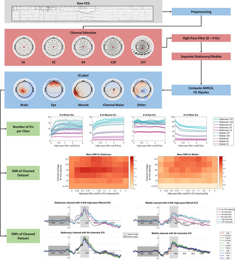
Schematic overview of the processing pipeline. Blue boxes mark processing steps which were executed identically for all datasets, red boxes mark a selection of conditions, green boxes mark final quality measures. Steps are described in section Processing pipeline
2.2.1 PreprocessingData from both conditions was first appended and individual channel locations were loaded. Raw EEG data were then low-pass filtered to the new Nyqvist-frequency to prevent aliasing (zero-phase Kaiser-windowed sinc Finite Impulse Response (FIR) filter, Kaiser beta = 5, cutoff = 112.5 Hz, stopband = 125 Hz, transition bandwidth = 25 Hz, default when using the pop_resample function of EEGLAB) before being resampled to 250 Hz. Subsequently, bad channels were detected manually to remove strong outliers which were then interpolated (e.g. channels heavily contaminated by line noise, transient artifacts from electrode shifts, or strong drifts, 17.6 channels on average, SD = 9.5). Lastly, channels were re-referenced to the average reference.
2.2.2 Channel selectionIn the next step, we selected channels of the dataset to be included in the analyses. These included either all channels, using the full equidistant setup with 129 scalp and 28 neck electrodes or a subset of only the scalp electrodes, resulting in a 128, 64, 32, and a 16 channel scalp setup. The subsampled channel layouts of 64 and less channels were chosen such that the whole head was covered while the mean of the channel locations remained within 1 cm of the mean of the 128 channel layout. Since the data contained free eye movements, the two electrooculogram (EOG) electrodes below the eyes were kept for all setups. Earlier testings pointed toward different results when using a more dorsal channel layout in the 16 channel recordings, which is why an additional channel layout was tested. To not inflate the results section, the effects of this layout can be found in the supplementary material. The channel subset selection was identical for all participants, see Figure 2 for an exemplary visualization of the channel layouts. These data constituted the basic datasets ("datasets A").
2.2.3 High-pass filteringIn order to compare the impact of different high-pass filter frequencies on ICA decompositions, the five datasets A were filtered with a zero-phase Hamming window FIR-filter (EEGLAB firfilt plugin, version 1.6.2) with varying cut-off frequencies. In many cases, it is advisable to specify the filter order in detail to achieve maximal control of the process (see Widmann et al., 2015) for a practical guide to filtering EEG data). The filter passband-edge defines where signal attenuation begins, the cut-off frequency is the frequency where the signal is attenuated by 6 db and can be regarded as the frequency where the filter starts to have a noticeable effect. The transition bandwidth is double the difference between passband-edge and cut-off frequency and is specified by the filter order. The stopband-edge is the passband-edge minus the transition bandwidth and can be regarded as the frequency where the signal attenuation reaches its full effect. At this point, it should be noted that in EEGLAB filters are specified by passband edge and follow a heuristic to find a suitable filter order (and thus transition bandwidth) depending on the frequency. For example, a default 1 Hz filter as used by EEGLAB routines has a transition bandwidth of 1 Hz and a cut-off of 0.5 Hz, whereas a 3Hz filter has a transition bandwidth of 2 Hz and a cut-off frequency of 2 Hz. For the present study, we used a constant filter order of 1,650 to ensure comparability, resulting in a transition bandwidth of 0.5 Hz independently of the passband-edge. 2 This means that a filter with a specified passband edge of 1 Hz and a transition bandwidth of 0.5 Hz leads to a cut-off frequency of 0.75 Hz and a stopband frequency of 0.5 Hz. In the further course of this paper, we use the cut-off frequency to specify the filter. As the literature suggests, we focused our analysis on lower frequencies. Since the transition bandwidth was 0.5 Hz, the lowest cut-off frequency that could be applied was 0.25 Hz. We then increased the frequency in steps of 0.25 Hz for lower frequencies up to 1.5 Hz, then in steps of 0.5 Hz up to 3 Hz, and added a 4 Hz filter as the highest frequency. Additionally, we added an analysis without any additional filtering (“0 Hz”) for comparison. This resulted in 11 different filter settings for all of the datasets A.
2.2.4 Data selectionAfter filtering, segments in the data which were not part of the experiment were rejected and subsequently a manual cleaning followed where the data were scored for strong artifacts (on average 11.1% of the experiment data was removed, SD = 5.6%). The marked timepoints were saved and rejected from all filtered datasets. The separation of the stationary and mobile experimental conditions was made based on the event markers present in the data. Importantly, to ensure comparability, both the stationary and mobile conditions had to be of the same length. As a consequence, the longer dataset was cut to the length of the shorter dataset (on average, datasets were 27 min long, SD = 5.8 min). Overall, this resulted in 110 datasets per subject composed of 2 (movement conditions) × 5 (channel montages) × 11 (filter cutoff) that entered an ICA decomposition.
2.2.5 Independent Component AnalysisAll final 2090 datasets (110 datasets × 19 participants) were then decomposed using the AMICA algorithm (Palmer et al., 2011). AMICA was chosen since it is considered the best ICA algorithm (see section Achieving an optimal decomposition) and is widely used by different research groups. Although the impact of filtering has been evaluated for algorithms other than AMICA, AMICA itself was not often subject to these investigations. We used one model and ran AMICA for 2000 iterations on all datasets. Since we interpolated channels previously and used an average reference for our datasets, we also let the algorithm perform a principal component analysis rank reduction to the number of channels minus 1 (average reference) minus the number of interpolated channels. All computations were performed using four threads on machines with identical hardware, an AMD Ryzen 1,700 CPU and 32GB of DDR4 RAM. Overall, computation time amounted to 4,340 hr for all participants and datasets.
2.2.6 Dipole fittingSubsequently, for every resulting IC, an equivalent dipole model was computed as implemented by the DIPFIT plugin for EEGLAB. For this purpose, the individually measured electrode locations of every participant were warped (rotated and rescaled) to fit a boundary element head model based on the MNI brain (Montreal Neurological Institute, MNI, Montreal, QC, Canada). The dipole model includes an estimate of IC topography variance which is not explained by the model (residual variance, RV).
2.2.7 Transfer of AMICA and equivalent dipole model structuresSince the final quality measures of the resultant AMICA decomposition needed to be computed on comparable unfiltered data to allow for a direct comparison of ICs, we copied the resulting weight matrices of the AMICA and the equivalent dipole model back to dataset A. This also allowed an automatic IC classification based on ICLabel (Pion-Tonachini et al., 2019) to be performed on data containing the complete spectrum which increases classification accuracy. Subsequently, the data were cleaned and separated into the two movement conditions (identical to section Data selection).
2.2.8 Automatic component classificationThe next part of the processing was the automatic classification of ICs using the ICLabel algorithm (Pion-Tonachini et al., 2019). ICLabel is a classifier trained on a large database of expert labelings of ICs, which classifies whether or not ICs are of brain or non-brain origin, including eye, muscle, and heart sources as well as channel and line noise artifacts and a category of other, unclear, sources. The class probability is provided allowing both for a more fine-grained analysis of probabilities and a classic popularity vote classification. Classifying based on a class probability threshold per class can be beneficial when the focus of interest lies mainly on one class, but it can also lead to ICs which have zero or more than one class labels assigned. Since we were interested in comparing the different classes, we used the popularity vote for our analysis. As a result, ICs received the class with the maximal probability as their class label. Two versions of the ICLabel algorithm exist: i) the default version which uses the IC activity spectrum (1-100Hz), IC topography, and IC activity autocorrelation as features for classification, and ii) the lite version which does not take autocorrelation into account. The latter is faster to compute and uses less RAM, especially for larger datasets, and although the classification of brain ICs can be slightly better in the default version, classification of other sources like eyes and muscles can be better using the lite version. Hence, we ran ICLabel twice using both versions but focus our analysis on the lite version. 3 See Figure 2 for example patterns of the most important classes.
2.2.9 Automatic selection of parietal componentsIn addition to the ICLabel classification, we automatically selected one parietal IC for each decomposition, based on a topographic weight map. To allow automatic selection of this parietal component, we took the first 10+ number of ICs/ 3 ICs with a RV of <10% into account. The analysis of a specific brain IC allowed for an additional investigation of the impact of the preprocessing independent of ICLabel. Additionally, this allowed for investigating the effect of channel density, filtering, and movement on specific scalp topographies as opposed to a general decomposition quality. This can be important when using ICA to examine the data on the source level, for example in a parietal region of interest. See Figure 2 for an example parietal pattern. The low-density layouts with 16 and 32 channels were excluded from this analysis because parietal patterns could not be detected reliably. Additionally, two subjects had to be excluded even in the high-density layouts because the algorithm failed to reliably detect a parietal pattern.
2.3 Quality measuresIn order to compare the decomposition quality, we extracted several features addressing both general and practical considerations.
First, we considered the ICLabel classifications. The focus of most EEG research lies on brain signal analysis and the removal of other sources that are considered artifactual contributions. In MoBI research, in contrast, analyzing muscle and eye activity as signals can be very important to make sense of the data and potentially to be used as a source of insight into cognitive processes. Hence, we were interested in the amount of brain, eye, and muscle ICs as signal sources, and the amount of other ICs as a proxy of general decomposition quality.
Additionally, we were interested in the residual variance of ICs after fitting an equivalent dipole model. The RV, especially of brain components, is an important measure to estimate the quality of a component (Delorme et al., 2012). A low RV means that the respective independent component is largely dipolar in nature, which in turn indicates more physiologically plausible sources that are more likely to be of brain origin, since the standard head models only include dipoles in the cortex. Often, this measure is used to separate brain ICs from other ICs where ICs with an RV <15% are treated as more likely originating in the brain. We were interested in the mean intra-class RV for the ICLabel classes as well as the mean RV of the parietal ICs.
Finally, as a practical measure for researchers, event-related-responses (ERPs) were computed for all datasets and further examined on their the signal-to-noise ratio (SNR). To this end, the data were pruned with ICA by removing all ICs that were classified as non-brain classes and only brain ICs were backprojected to the sensor level. In case no IC was classified as brain, the one with the highest brain probability was used (over all conditions, this occurred 16 times). Since the data were previously scored for strong artifacts in the time domain, only trials not containing these artifacts entered the ERP. The ERPs were computed at an electrode in equidistant layout which was positioned closest to the POz electrode in the standard layout (POz’). Importantly, to not distort the results we used no frequency filter on the data (as the ICA results were copied back to the unfiltered data), but only the spatial filter of the ICA. We then extracted epochs (−600 ms to +1,200 ms) around the trial-onset event (onset of the moving sphere) for which we expected a parietal late positive complex to occur, and removed the pre-stimulus baseline activity. The two mobility conditions (stationary, mobile) did not contain the same amount of events, as the stationary condition had to be cut short to fit in length to the mobile condition in which participants rotated back faster and thus were able to answer more trials within the same time. To ensure comparability between the conditions, we determined the minimal number of available events for both movement conditions per subject and used this number of events in both conditions to compute the ERPs. On average, 77.8 (SD = 18.2) epochs were used per subject and condition, and the final measures for signal and noise were computed. To this end, the mean amplitudes from 250 ms to 450 ms served as the signal which was divided by the standard deviation in the 500 ms pre-stimulus interval to compute the SNR (Debener et al., 2012).
3 RESULTSAs the effects are either clearly visible in the figures or a reflection of the arbitrarily chosen filter steps, statistical testing was not performed. Overall, the ICA decompositions were sensitive to the different preprocessing parameters. Figure 3 shows the results for the number of ICs in the Brain, Muscle, Eye, and Other, classes, as well as their mean RV. The results of the RV values of the parietal ICs can be seen in Figure 4. Finally, the practical quality measures of ERPs and SNR values can be found in Figure 5.

Results for the ICLabel classifications (n = 19). Shaded areas depict the standard error of the mean. 0 Hz refers to no additional filter being applied before computing ICA. Note the logarithmic scaling of the abscissa with grid lines for each available filter frequency. Top row: amount of ICs per class, bottom row: mean residual variance (RV) per class.

Residual variance (RV) of the parietal patterns (n = 17). Shaded areas depict the standard error of the mean. Only channel montages of 64 and more channels were considered. 0 Hz refers to no additional filter being applied before computing ICA. Note the logarithmic scaling of the abscissa with grid lines for each available filter frequency.

Practical quality measures (n = 19). Top: Signal-to-noise ratios (SNRs) of the event-related-responses (ERPs) computed on uncleaned data and data that were cleaned with ICA by removing all non-brain ICs as classified by ICLabel. ERPs were computed on the POz’ electrode for the trial-onset event. Note that as the ICA results were copied back to the unfiltered datasets prior to ERP computation, the datasets themselves only differed in the ICA decompositions that were used for cleaning, no frequency filter was applied before computing the ERPs. SNR was defined as the mean amplitude in the 250 ms–450 ms interval divided by the standard deviation in the 500 ms pre-stimulus interval. 0 Hz refers to no additional filter being applied before computing ICA. Bottom: Corresponding ERPs, plotted either for different channel montages and a fixed filter cutoff frequency used before computing ICA (columns of SNR plots, a, b, e, f), or different cutoff frequencies and a fixed channel montage (rows of SNR plots, c, d, g, h).
Clear differences could be observed between the stationary and mobile data. The stationary data contained more brain ICs and less muscle ICs than the mobile data (see Figure 3), and additionally, the mobile data contained more ICs classified as "other". Interestingly, the number of eye ICs did not differ between the mobility conditions. A larger RV of brain ICs could be observed in the mobile condition, however, this difference was not very large. Considering the parietal ICs specifically (see Figure 4), the mobile condition consistently exhibited a slightly higher RV than the counterparts in the stationary condition. The SNR of the ERPs was considerably greater in the stationary condition than in the mobile condition (see Figure 5), and the shape of the ERP in the two mobility conditions was different, with a larger late positive peak including a steeper offset in the stationary condition.
The ICA decomposition was also clearly influenced by the channel montage, with generally more ICs being present in each class in higher channel densities. This was evident also in the number of brain ICs, but even with 16 channels there were still ICs classified as brain. Importantly, the difference in brain ICs between montages with different channel densities appeared less pronounced than the difference in muscle and other ICs, indicating a possibly more pronounced stability of the brain ICs. Note that the maximum of brain ICs was not reached with the montage containing the neck band (157 channels), but with 128 scalp channels. This was true for both mobility conditions, but the detrimental effect of the neck band was less pronounced in the mobile condition. The number of eye ICs was stable across channel montages, with densities of 64 channels and upward containing four eye ICs, the 32 channel montage containing three eye ICs, and only the 16 channel montage containing only two ICs classified as reflecting eye movement activity. The RV of channel montages with fewer channels was lower in general. The 16 channel montages reached RV values of <10% in most cases, including not only physiological, but also other ICs. The difference between the channel montages were more pronounced for muscle and other ICs than for brain ICs, which means that the difference in RV values between brain and non-brain ICs was larger when using more channels. In the parietal ICs, the 157 channel montage showed a general increase of RV (around 2 percentage points) above the 128 and 64 channel montages, whereas only a slight increase could be observed in the 128 channel montage over the 64 channel montage. Interestingly, when looking at the SNR and the ERP waveforms, the 64 channel montage already led to very good or the best results and cleaning the data with ICA based on 32 channels already led to a substantial improvement in SNR. The improved SNR values did not come at the cost of increased standard deviations which would indicate more outliers. On the contrary, the standard deviation of the SNRs was generally lower when the data were cleaned with ICA. Visual inspection of the ERPs showed improvements already for 16 channels when cleaned with ICA, but the ERP waveform, especially in the mobile condition, was more similar to the uncleaned ERP than to the ERP of the 32 channels condition. However, employing a channel layout more focused on dorsal electrodes led to an improvement of the SNR and ERP waveforms (see supplementary material).
The high-pass filter applied before computing ICA had a considerable influence as well. For brain and muscle ICs an increase in the number of ICs in these classes with increasing high-pass frequencies could be observed, especially when compared to the data without additional filter (“0 Hz”). The number of eye ICs appeared to be insensitive to high-pass filtering, whereas the number of other ICs dropped with increasing filter frequency. The effect of filtering also exhibited a ceiling (brain/muscle ICs) or floor (other ICs) effect, where a filter higher than 1–2 Hz did not affect the results any further. The number of muscle ICs increased a little slower, approaching an optimum from 2Hz onward and continued to increase even up to 4 Hz cut-off (maximum filter applied). The RV of brain ICs appeared relatively stable across different filter frequencies, implying that an increased number of brain ICs did not coincide with classifying less dipolar ICs as originating in the brain. The mean RV of brain ICs ranged from 3% (stationary condition with 16 channels) to 15% (mobile condition with 157 channels). RV values of muscle and other ICs droppped with increasing filter frequency up to 1 Hz, which was more noticeable with higher channel densities. In the parietal ICs, a slightly different pattern was observed, where the RV did not approach a floor asymptote, but increased again after reaching the minimum around 1 Hz. This inverted U-shape with increasing filter frequencies could also be observed for the SNR measures of the ERPs and the ERP waveforms themselves, where mid-range filters showed a larger late positive signal, not only in the range used for the SNR computation (250 ms to 450 ms post-stimulus) but continuing until around 600 ms post-stimulus. In the parietal ICs, the already small difference between the 64 and the 128 channel montage disappeared at the optimal filter frequency. The SNR in higher channel densities generally required a higher filter to reach its maximum which could also be seen in the ERPs themselves.
Finally, the effects of filter and mobility conditions appeared to interact as well. For the number of brain ICs, the necessary filter to reach the maximum showed a marked difference between stationary and mobile data: The maximum number of 17.2 brain ICs in the stationary condition was reached with 128 channels and a 1 Hz filter. In contrast, the maximum of 12.7 brain ICs in the mobile condition was reached also with 128 channels but requiring a filter of 2.25 Hz. The SNR of the ERPs also showed that in the mobile condition a higher filter led to the best results. As expected from the SNR values, the ERP waveforms with the highest late positive values in the mobile condition were the ones cleaned with ICA computed on higher filtered data, especially noticeable with 128 channels where the maximal late positive peak occurred with the 2.25 Hz filter in the mobile condition as opposed to 1.25 Hz in the stationary condition.
留言 (0)