1 INTRODUCTION 1.1 Navigation assistance systems and spatial knowledge acquisition

Navigating and orienting in our environment are fundamental aspects of every-day activities. Common navigation tasks vary with regards to the distance traveled and familiarity with the environment. Accordingly, navigation tasks range from commuting to work, or grocery shopping to touristic trips, or long hikes to explore new areas. Increasingly, technology, i.e., navigation assistance systems, facilitates or even take over parts of these spatial orienting tasks. The frequent use of navigation aids, however, was shown to be associated with decreased processing of the environment (Ishikawa et al., 2008; Münzer et al., 2006) and to be adverse to the ability to successfully use spatial strategies when no navigation aid is available (Dahmani & Bohbot, 2020).

In previous studies, we demonstrated that the use of commercial navigation instructions that highlight an “intersection” (e.g., “Turn left at the next intersection!”) leads to a decrease of landmark knowledge. This was especially detrimental regarding knowledge of landmarks at decision points with route direction changes (Gramann et al., 2017; Wunderlich & Gramann, 2018, 2020). These studies further demonstrated the successful incidental acquisition of landmark and route knowledge when landmark-based rather than standard instructions were used. The experimental setups in these studies ranged from simulated driving through a virtual world (Wunderlich & Gramann, 2018) to interactive videos of walking or actually walking through the real-world (Wunderlich & Gramann, 2020). The results revealed higher amplitudes of the event-related late positive component (LPC) at parietal leads with the cued recall of landmark pictures. The increased LPC was interpreted as reflecting the recollection of more spatial information which corresponded to better cued recall performance observed for landmark-based navigation instructions (Wunderlich & Gramann, 2018). Even though these studies provided new insights into spatial knowledge acquisition when assistance systems were used for navigation, they all addressed spatial knowledge acquisition after the assisted navigation phase providing no further insights into incidental spatial knowledge acquisition during navigation.

1.2 Investigating brain activity during navigation in real-world studies

Overcoming the restrictions of established brain imaging methods (Gramann et al., 2011; Makeig et al., 2009), new mobile brain imaging devices allow for recording human brain activity during active navigation and in the real-world providing high ecological validity (Park et al., 2018). Real-world navigation includes natural interaction with a complex, dynamically changing environment and other social agents, as well as realistic visuals and soundscapes. However, mobile EEG recordings come with several problems. First, active movement through the real-world is associated with increasing noise in the recordings (Gramann et al., 2014). The EEG records data on the surface of the scalp that is the result of volume conducted brain and non-brain sources. The latter include biological sources (e.g., eye movement and muscle activity) as well as mechanical and electrical artifacts (e.g., loose electrodes, cable sway, electrical sources in the environment). A second problem lies in a multitude of external and internal events that are impossible to control but are naturally present when the real-world is used as an experimental environment to investigate cognitive phenomena. Some of these events might provoke artifactual activity with respect to the phenomena of interest (e.g., a startle response to a car horn or suddenly appearing pedestrians). Finally, tests in the real-world do not allow for the control of the number and timing of the events of interest that are usually presented in high numbers for the analysis of event-related brain activity (Luck et al., 2000).

The problem of inherently noisy data can be addressed by blind source separation methods such as independent component analyses (ICA, Bell & Sejnowski, 1995; Makeig et al., 1996). Removing non-brain sources from the decomposition allows for back-projecting only brain activity to the sensor level, using ICA as an extended artifact removal tool (Jung et al., 2000). The second problem, the multitude of random events, might be overcome by an averaging approach of event-related potentials (ERPs) to average out EEG activity that was not related to the processes of interest. However, to do so, the third problem has to be solved and a sufficiently high number of meaningful events has to be found for event-related analyses and the related activity extracted and separated from other or overlapping activity (Ehinger & Dimigen, 2019).

1.3 Eye movement-related events and potentials

Physiological non-brain activity captured in the mobile EEG can be used as a source of meaningful events for the analyses of ERPs. Using such activity is non-intrusive to the ongoing task (Bentivoglio et al., 1997). and naturally occurring physiological events like eye blinks and saccades allow to parse the EEG signal into meaningful segments as they covary with visual information intake (Berg & Davies, 1988; Kamienkowski et al., 2012; Stern et al., 1984). Saccades suppress visual information intake starting 50 ms preceding a saccade-onset as well as during the saccade. Thus, each fixation following a saccade represents the onset of visual information intake. Event-related potentials using saccades can be related to either saccade onset, peak velocity, or saccade offset, with the latter being equivalent to the fixation-related potentials (fERP). Saccade-related brain potentials (sERP) were used in many previous studies (Gaarder et al., 1964; Rämä & Baccino, 2010), especially in research investigating reading and text processing (Baccino, 2012; Dimigen et al., 2011; Marton & Szirtes, 1988) or visual search (Kamienkowski et al., 2018; Kaunitz et al., 2014; Ossandón et al., 2010).

The sERP starts with the parietal presaccadic spike potential, which represents the execution of the saccade as well as its attentional/motivational value (Sailer et al., 2016). The posterior positive component 80 ms from the saccade offset is labeled lambda response (Kazai & Yagi, 2003) which was shown to be sensitive to properties of the visual stimulus like luminance or contrast (Dimigen et al., 2011; Gaarder et al., 1964; Kaunitz et al., 2014; Kazai & Yagi, 2003). The sensitivity of the lambda response to the properties of incoming visual information as well as its close cortical origin renders the lambda response comparable to the P1 in stimulus-evoked ERPs (Kazai & Yagi, 2003). Thus, the P1 and lambda response seem to be elicited by the same perceptual process (Kaunitz et al., 2014). The subsequent P2 of the sERP at posterior leads was shown to be sensitive to the processing of context information (Marton & Szirtes, 1988) and semantic meaning of text information (Simola et al., 2009). Simola et al. (2009) showed a right hemispheric dominance of the P2 component when processing words versus non-words. In visual search, the parietal P2 demonstrated decreased amplitudes when fixating targets compared to distractors (Kamienkowski, Navajas, et al., 2012). In a later time window starting at 380 ms Kamienkowski et al. (2012) showed a positive component for targets only at frontal leads.

In contrast to saccades, blinks produce a longer interruption of the visual input stream (for a review see Stern et al., 1984). Despite startle, invasive external events or dry eyes, there are at least three different factors determining the timing of blink generation. First, in order to keep the efficiency of the visual input channel high, and to reduce interruptions in the visual information stream, blinks are combined with other eye movements (Evinger et al., 1994). Second, blinks likely occur after a period of blink suppression (e.g., during attention allocation) or when the processing mode changes. Thus, they can mark the end of an information processing chain (Stern et al., 1984). Third, in very structured tasks using for example stimulus-response pairs, blinks show a temporal relationship to stimulus presentation (Stern et al., 1984). Like saccades and fixations, blinks have been used for extracting event-related potentials (bERP). The bERP was shown to be sensitive to the parameters of the experimental environment or characteristics of the current task (Berg & Davies, 1988; Wascher et al., 2014). The long preceding pause of incoming visual information might make bERPs more similar to ERPs. In addition, the increased likelihood for blinks at the end of information processing steps qualifies the bERPs during natural viewing as a valuable source of insight about visual information processing and underlying cognitive processes.

Berg and Davies (1988) stated that the time point zero in bERPs comparable to ERP research is when the eyelid uncovers the pupils. This happens about 100 ms after the blink maximum and thus qualifies the occipital P200 and N250 referenced to the blink maximum as candidates to represent comparable processes like the P1/N1 complex of the stimulus-evoked potential. Based on the interpretation of the visual evoked activity in traditional ERP studies, the P200 in the bERP (P1 in ERP studies) would reflect an exogenous component related to the sensory processing of attended incoming visual information which is influenced by stimulus parameters like contrast. The N250 in the bERP (N1 in ERP studies) would be related to the allocation of attention to task-relevant stimuli and discrimination of stimulus features (Luck, 2005; Luck et al., 1990). A fronto-central P100 of the bERP was shown to be less pronounced and the following N200 to be more pronounced in a cognitive task when compared to a physical task or rest (Wascher et al., 2014).

Regarding later evoked components of the bERP, Berg and Davies (1988) described the posterior P300 to be more pronounced when subjects blinked under light as compared to blinking in darkness. In the latter case, the bERP P300 was nearly absent, implying that this P300 reflects the processing of incoming visual information. Accordingly, Wascher et al. (2014) found the posterior P300 to be most pronounced during rest, followed by the cognitive task and least pronounced during the physical task reflecting amplitude modulation due to information processing. The waveform of the component reminds of the P300 at posterior leads in traditional ERP studies and seems to be composed of several sub-components underlying different cognitive processes.

1.4 Research goal and hypotheses

In this paper, we describe a means to deal with the previously specified issues arising from collecting mobile EEG during an ongoing task in the real-world. We show how both blink- and saccade-related potentials alongside gait-related activity in uncontrolled real-world environments can be extracted from IC source time series. These events can subsequently be analyzed to gain deeper insights into the ongoing brain activity accompanying information processing in the real-world.

In the present study, we used this approach to investigate human brain activity during assisted pedestrian navigation using standard or landmark-based auditory turn-by-turn instructions. We investigated how navigation instructions might change visual information processing and incidental spatial knowledge acquisition. We recorded and analyzed brain activity in the real-world, while participants navigated through the city of Berlin and were subsequently tested on their acquired spatial knowledge. Based on previously observed increased LPCs for landmarks presented in a cued-recall task after navigation with landmark-based instructions, we expected landmark-based navigation instructions to generally shift attention toward information in the environment relevant for navigation. The accompanying improved spatial knowledge acquisition was assumed to lead to a better performance in the follow-up spatial tasks.

To investigate how navigators process the environment during assisted navigation, we used blink- and saccade-related potentials. These were extracted during the entire navigation task and analyzed separately for navigation periods at intersections where auditory navigation instructions were provided and periods were navigators walked straight segments of the route without navigation instructions. Eye movement-related potentials were expected to reveal differences between navigation instruction conditions, especially at intersections. Group differences during straight segments would indicate a general change in visual information processing. While this was an explorative study investigating eye movement-related brain potentials in a real-world navigation task, previous ERP studies and studies using eye movement-related brain activity in established laboratory settings allowed for some hypotheses about differences in evoked potentials. Based on earlier laboratory studies, we expected group differences in early visual components at posterior leads reflecting instruction-dependent visuo-attentional processes. Furthermore, we expected more pronounced later components over parietal leads representing information integration and memory encoding, while late potential differences over fronto-central leads were expected to reflect a different involvement of higher cognitive processes.

2 MATERIALS AND METHODS 2.1 Participants

The data of 22 participants (11 women) were analyzed with eleven participants in each navigation instruction condition. Their age ranged from 20 to 39 years (M = 27.4, SD = 4.63 years). Participants were recruited through an existing database or personal contact and received either 10 Euro per hour or course credit. All had normal or corrected to normal vision and gave informed consent prior to the study which was approved by the local research ethics committee of the Institute for Psychology and Ergonomics at the Technische Universität (TU) Berlin. Before the main experiment, participants filled out an online questionnaire to determine if they were familiar with the area where the navigation task would take place (Wunderlich & Gramann, 2020). After navigating the route, participants were again asked whether they had been familiar with the navigated route. In case participants stated familiarity with more than 50% of the route, they were excluded from the second part of the experiment and data analysis. In the final sample of 22 participants, familiarity ratings ranged from 0% to 40% (M = 9.52%, SD = 12.2%).

2.2 Study design and procedure

The experiment consisted of two parts and lasted approximately 3 hr in total. In the first part, participants walked a predefined route through the district of Charlottenburg, Berlin in Germany, using an auditory navigation assistance system. In the second part, directly after the navigation task, participants were transported back to the Berlin Mobile Brain/Body Imaging Lab (BeMoBIL) at TU Berlin to run different spatial tests. Participants had not been informed about the spatial tasks and that they would be tested on the environment after the navigation task.

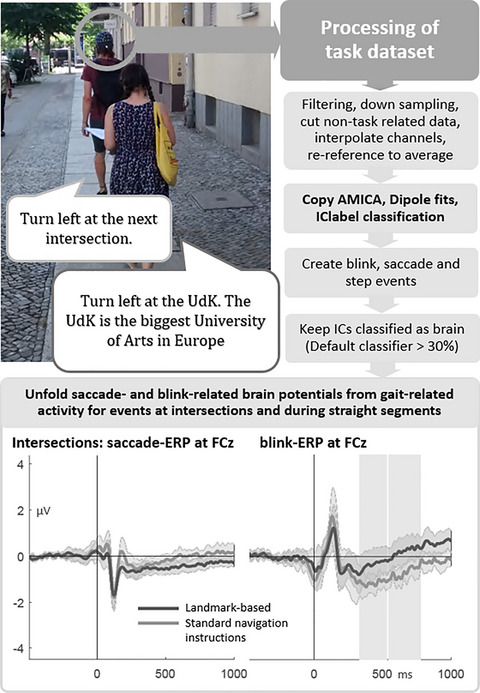
During the navigation task, participants followed the auditory navigation instructions to navigate along a 3.2 km long, predefined, unfamiliar route with twenty intersections. There were two groups of participants, either receiving standard or landmark-based navigation instructions prior to each intersection. Based on previous results (Gramann et al., 2017; Wunderlich & Gramann, 2018, 2020), landmark-based instructions referenced a landmark at each intersection and provided more detailed information about this landmark. One example of navigation instruction for this landmark-based condition was “Turn left at the UdK. The UdK is the biggest University of Arts in Europe.” This contrasted with the standard navigation instruction condition that used instructions like “Turn left at the next intersection.” Previous to the navigation task, it was pointed out to the participants that they should follow the auditory turn-by-turn instructions and be aware of other traffic participants, especially while crossing streets. Furthermore, in case they feel lost, they were asked to stop and turn to the experimenter who was shadowing the participant with two to three meters distance. The presence of the experimenter ensured the participant's safety as well as the correct course of the route. The experimenter manually triggered the auditory navigation instructions using a browser-based application on a mobile phone. Participants received the auditory navigation instructions by Bluetooth in-Ear headphones at predefined trigger points in the environment. After walking for approximately 40 min, the participants arrived at the end of the route. There, they were instructed to rate their subjective task load during navigation using the National Aeronautics and Space Administration Task Load Index (NASA-TLX; Hart, 2006; Hart & Staveland, 1988). Additionally, they filled in three short questions regarding their prior knowledge of the route.

The second part of the experiment took place at the BeMoBIL. There, the first task was to draw a map of the route on an empty sheet of paper (DIN A3) and secondly to solve a cued-recall task. In the latter task, sixty landmark pictures were given as cues and the required response included the respective route direction. The randomly shown landmarks had been either located at intersections (and mentioned in the landmark-based navigation instructions) or at straight segments of the route (without navigation instructions), or they were similar in appearance but not part of the previously navigated route. In the end, demographic data as well as individual navigation habits, and subjective spatial ability ratings using the Santa Barbara Sense of Direction Scale (SBSOD; Hegarty et al., 2002) and the German questionnaire Fragebogen Räumliche Strategien (FRS; Münzer et al., 2016; Münzer & Hölscher, 2011) as well as perspective taking (PTSOT; Hegarty & Waller, 2004) were collected.

2.3 Electroencephalography 2.3.1 EEG data collection

The EEG was recorded continuously during the navigation task and the subsequent laboratory tests using an elastic cap with 65 electrodes (eego, ANT Neuro, Enschede, The Netherlands). Electrodes were placed according to the extended 10% system (Oostenveld & Praamstra, 2001). All electrodes were referenced to CPz and the data were collected with a sampling rate of 500 Hz. One electrode below the left eye was used to record vertical eye movements. Time synchronization and disk recording of the EEG data stream and the event marker stream from the mobile application and task paradigm was performed using Lab Streaming Layer (LSL, https://github.com/sccn/labstreaminglayer; Accessed on November 1, 2020).

2.3.2 EEG data processing

For EEG data processing, the MATLAB toolbox EEGLAB was used (Delorme & Makeig, 2004). The raw EEG data of both the navigation phase and the cued-recall task were high pass filtered at 1 Hz, low pass filtered at 100 Hz using the EEGLAB filter function eegfilter(), and subsequently resampled to 250 Hz (see Figure 1, left column). The pre- and post-task phases of the EEG data were removed. Afterward, the two separate datasets of each participant were merged into one dataset and channels that were subjectively judged as very noisy, flat, or drifting were manually rejected (M = 3.79, SD = 1.77, Min = 1, Max = 8). Continuous data cleaning was applied twice using the pop_rejcont() function for frequency limits from 1 to 100 Hz and default settings for all other parameters. 1 Rejected channels were interpolated using a spherical spline function and the data were re-referenced to the average reference. Time-domain cleaning before interpolation and re-referencing targeted artifacts on a single channel level prohibiting the inflation of single noisy channels when re-referencing to average reference. A second-time-domain cleaning was applied to remove the remaining artifactual data.

EEG data processing from raw data to ICA computation (left) and from raw task data to the use of the unfold toolbox (right). Additional analysis steps in the ICA preprocessing have white boxes to emphasize the otherwise parallel processing

Subsequently, the data were submitted to independent component analysis (ICA, Makeig et al., 1996) using the Adaptive Mixture ICA (AMICA, Palmer et al., 2011). The resultant independent components (ICs) were localized to the source space using an equivalent dipole model as implemented in the dipfit routines (Oostenveld & Oostendorp, 2002). Finally, the resultant ICs were classified as being brain, muscle or other processes using the default classifier of IClabel (Pion-Tonachini et al., 2019).

The original sensor data were preprocessed using identical processing steps as described above save different filter frequencies and no time-domain data cleaning (see Figure 1, right column). The respective weights and sphere matrices from the AMICA solution were applied to the preprocessed navigation dataset. In addition, the equivalent dipole models and IClabel classifications for each participant and IC were transferred to the respective task dataset allowing for the extraction of events based on the complete duration of the task.

2.4 Event extraction from IC time course

The event extraction is summarized in Figure 2. Blinks were identified using one IC from the individual decompositions that reflected vertical eye movements as described in Lins et al. (Lins et al., 1993). In case of more than one candidate for the vertical eye IC, the component showing a better signal to noise ratio for blink deflections and/or less horizontal eye movement was chosen based on subjective inspection.

Analysis steps for the extraction of events from the respective IC activation(s): blink (left), saccade (middle), and step events (right). The respective parameters for the findpeaks() functions can be found in the text

For detecting blinks, the associated component activation time course was filtered using a moving median approach (window size of twenty sample points equaling 80 ms). Moving median approaches smooth without changing the steepness of the slopes in the data (Bulling et al., 2011). To allow for automated blink peak detection, all individual IC time courses were standardized to a positive peak polarity. Peak detection was performed using the MATLAB function findpeaks() applied to the filtered IC activation. Parameters used were a minimal peak distance of 25 sample points (100 ms) to avoid directly following blinks to be selected. Further, peaks were restricted to a minimal peak width of 5 (20 ms) and maximal peak width of 80 sample points (320 ms) to suppress potential high-amplitude artifacts or slow oscillations from being counted as a blink. The following two parameters were automatically defined for each dataset individually to take care of interindividual differences in the shape of the electrical signal representing a blink: the 90-percentile of the filtered activation data was applied to define a threshold of minimal peak prominence. This parameter ensured the successful separation of detected peaks from the background IC activity. For the absolute minimal peak height, a threshold was defined using the 85-percentile of the filtered activation data. For each peak location, an event marker with the name blink was created in the EEG dataset at the time point of maximum blink deflection.

Saccades were identified using two ICs from the individual decompositions that reflected vertical and horizontal eye movements, respectively (according to Lins et al., 1993). Vertical eye movement ICs were the same as used for blink detection. For the horizontal eye movement ICs, the IC with the most characteristic scalp map and rectangular activity in the activation time course reflecting horizontal eye movements was chosen based on subjective inspection. The associated component activation time courses were filtered using a moving median approach (window size of 20 sample points equaling 80 ms). The electrooculogram (EOG) activity was calculated using the root mean square of the smoothed time courses (Jia & Tyler, 2019). For saccade maximum velocity detection, the first derivative was taken and squared to increase the signal-to-noise-ratio. The function findpeaks() was applied to the squared derivative of the EOG activation. Parameters used were a minimal peak distance of 25 sample points (100 ms). Peaks were restricted to a minimal peak width of 1 (4 ms) and maximal peak width of 10 sample points (40 ms). The 90-percentile of the squared derivative of the EOG was applied for minimal peak prominence as well as for the minimal peak height threshold. In case identified peaks were closer than 30 sample points (120 ms) to a blink event, these peaks were not taken for saccade event extraction to avoid taking saccades into account that appeared during eyes closed periods. For each of the remaining peaks, an event marker called saccade was created in the EEG dataset at the time point of maximum saccade velocity (middle of the saccade).

Gait-related EEG activity was identified based on IC activation time course, scalp maps, and spectra from each individual decompositions. Up to two ICs were chosen manually that reflected gait cycle-related activity as described previously in studies comparing measures of kinematics and EEG activity (Jacobsen et al., 2020; Kline et al., 2015; Knaepen et al., 2015; Oliveira et al., 2017; Snyder et al., 2015). No filtering or smoothing was applied to the associated component activation time courses that showed a pronounced waveform at approximately 2 Hz. Inverting of time courses for some ICs was performed to align peak amplitudes on top of the slow-wave maxima. To extract single steps of the gait cycle, findpeaks() was applied to both IC activations consecutively. Peaks were restricted to a minimal peak width of 5 (20 ms) to take advantage of the high-frequency part and maximal peak width of 150 sample points (600 ms) to detect the slow-wave peaks. Minimal peak distance was set to 100 sample points (400 ms) to avoid that the high-frequency part and the slow-wave peak were both used for event extraction. The 80-percentile of the IC activation time course was applied for minimal peak prominence and as a threshold for minimal peak height. In case of step events identified in the two ICs being closer than 50 sample points (200 ms) one of the respective events was not taken into account for event generation. For each remaining detected peak, an event marker named step was created in the EEG dataset.

Afterward, every dataset was visually checked to validate blink, saccade, and gait events according to previous reports (Kline et al., 2015; Lins et al., 1993). To enable the comparison of blink- and saccade-related brain activity in different phases of the navigation task, we included different labels according to the task phases. The first event type was labeled baseline in case the event appeared before the first navigation instruction and thus was unaffected by the navigation instruction conditions. This baseline phase lasted on average six minutes (M = 352s, SD = 200 s). A second event type was labeled intersections in case the event took place within the 15 s following the onset of each of the twenty navigation instructions (in sum 300 s). The event type straight segments were used for all other remaining events in the navigation phase. On average, the time interval between two navigation instructions was 123 s. The number of events in each category can be seen in Table 1.

TABLE 1. Number of blink, saccade, and step events for all participants and separated by navigation instruction condition and navigation phase Number blink events Number saccade events Step Baseline Intersections Straight segments Baseline Intersections Straight segments All Standard instruction condition M 214 213 1,385 652 666 4,386 4,216 SD 142 81 592 224 113 1,104 1,033 Min 80 99 693 294 430 3,184 3,131 Max 572 355 2,730 996 857 6,808 6,878 Landmark based instruction condition M 183 193 1,236 559 794 4,307 3,994 SD 128 76 623 281 180 1,181 850 Min 68 89 384 184 366 1,893 1,762 Max 525 368 2,907 1,307 1,023 5,818 5,166 Abbreviations: M, mean; Max, Maximum; Min, Minimum; SD, standard deviation. 2.5 Source-based EEG data cleaning

Subsequently, all ICs with a classification probability lower than 30% in the category brain were removed from the dataset and the data were back-projected to the sensor level. This way the number of ICs per participant was reduced to M = 13.3 ICs (SD = 4.50 ICs, Min = 5 ICs, Max = 22 ICs). Considering the instruction conditions, this IC reduction did not lead to unbalanced numbers of ICs between the two instruction condition groups (standard: M = 13.1 ICs, SD = 5.12 ICs, Min = 5 ICs, Max = 22 ICs; landmark-based: M = 13.5 ICs, SD = 4.74 ICs, Min = 6 ICs, Max = 18 ICs).

2.6 Unfolding of event-related activity

The last data processing step on the single-subject level was the application of the unfold toolbox to the continuous data (Ehinger & Dimigen, 2019). This toolbox allows for a regression-based separation of overlapping event-related brain activity. As the extracted eye and body movement events in the navigation task overlapped with each other (Dimigen et al., 2011) and/or were temporally synchronized for some participants, it is a valuable tool to consider and control for overlapping ERPs and individual differences.

Following the published analysis pipeline of (Ehinger & Dimigen, 2019), we defined a design matrix with blink, saccade, and step events and 64 channels. We included the categorical factor navigation phase (baseline, intersections, straight segments) for the blink and saccade events into the regression formula: y = 1 + cat(navigation phase). For the step events, we only computed the intercept: y = 1. After applying the continuous artifact detection of the unfold pipeline and exclusion set to amplitude threshold of 80 µV, we time-expanded the design matrix according to the timelimits of −500 ms and 1,000 ms referring to the event timestamp. Afterward, we fitted the general linear model and extracted the intercept and beta values considering −500 ms to −200 ms for baseline correction (similar to Wascher et al., 2014).

While the blink and saccade-related potentials were considered as informative for the analysis of visual information processing during navigation, the step events were only used to control for their individual impact on the blink and saccade-related potentials. The intercept and beta values of the general linear model built the basis for a comparison between participants. Unfolded event-related potentials for all event types were computed for all electrodes and used for statistical analysis of group differences. The ERPs of participants within one navigation instruction condition and navigation phase were averaged and plotted alongside with twice the standard error of the mean (SEM) for FCz and as scalp map for five concatenated time windows.

2.7 Statistical analysis

We tested for group differences in individual and subjective measures using t tests of independent samples. The number of free-recalled landmarks in the sketch map and the sensitivity d′ of the cued-recall task were tested using each time a 2 × 2 mixed measure ANOVA with the between-subject factor navigation instruction condition (standard versus landmark-based) and the within-subject measure landmark location (intersections versus straight segments). The acquired route knowledge was compared between navigation instruction conditions for the landmarks at intersections using a t test of independent samples.

Statistical analysis on blink- and saccade-related brain potentials was performed for the interaction of navigation instruction condition (standard versus landmark-based) and baseline-corrected navigation phase (intersections versus straight segments). Group difference plots of the ERPs for both navigation phases were investigated to find time windows revealing significant differences between the navigation instruction conditions after the single-trial baseline ending at −200 ms. To define statistical significance between the unpaired values, the EEGLAB function statcondfieldtrip() was used. Due to this, a 10,000-fold permutation testing was applied followed by a cluster-based correction for family-wise error. If the returned probability corrected two-tailed p-value was below 0.05, the sample was marked as statistically significant.

3 RESULTS 3.1 Questionnaires

Using all questionnaire data, we checked for potential differences between the two experimental groups. When asking about the navigation assistance use, groups differed with respect to the use of navigation support (Item: “I use a navigation aid because I cannot find my way otherwise.”) The control group demonstrated less use of navigation aids (M = 2.73, SD = 2.05) compared to the landmark-based navigation instruction group (M = 4.45, SD = 2.11; t(20) = −1.94, p = 0.066, d = 0.83). No other items indicated differences between instruction groups (p's > 0.10). In addition, one item of the FRS targeting subjective orienting ability revealed a group difference. Navigators of the standard instruction group rated higher (M = 4.64, SD = 1.43) compared to the landmark-based navigation instruction group (M = 3.00, SD = 1.67; t(20) = 2.46, p = 0.023, d = 1.05) in the item: “If I walk through an unfamiliar city, I know the direction of the start and goal location.” All other items and the three factors of the FRS showed no significant differences (all p's > 0.171). The results of the SBSOD, the PTSOT, and the route familiarity after navigation showed no differences between the groups (all p's > 0.261).

Participants stated their task-related load after assisted navigation on six subscales of the NASA-TLX ranging from 1 to 100. The data revealed a difference of the two navigation instruction groups in the physical load assessment (standard: M = 38.5, SD = 23.5; landmark-based: M = 20.6, SD = 15.9; t(20) = 2.08, p = 0.050, d = 0.89) and a trend regarding the subjective mental load (standard M = 22.6, SD = 16.2; landmark-based: M = 37.5, SD = 18.4; t(20) = −2.01, p = 0.058, d = 0.86). All other subscales showed no difference between instruction groups (all p's > 0.177). There were no differences in walking speed between the instruction groups (standard M = 4.76 km/h, SD = 0.35 km/h; landmark-based: M = 4.86 km/h, SD = 0.34 km/h; t(20) = −0.68, p = 0.506).

3.2 Spatial knowledge acquisition

Free-recall of landmark knowledge was compared using a 2 × 2 ANOVA with the between-subject factor navigation instruction condition (standard versus landmark-based) and within-subject factor landmark type (intersections versus straight segments). The dependent variable analyzed was the number of correct landmarks marked in the sketch map. The main effect of navigation instruction condition (F(1,20) = 30.5, p < 0.001, η2p = 0.604) as well as the main effect landmark type were significant (F(1,20) = 31.0, p < 0.001, η2p = 0.608). The interaction effect also reached significance (F(1,20) = 25.9, p < 0.001, η2p = 0.564). Post hoc contrasts of the interaction revealed that the number of correctly drawn landmarks at intersections was higher for the landmark-based navigation instruction condition (M = 9.91, SE = 0.92, p < 0.001) when compared to the standard navigation instruction condition (M = 1.91, SE = 0.92). The number of correctly drawn landmarks at straight segments was comparably low across navigation instruction conditions (p = 0.721).

The performance of the cued-recall task was used to compute the dependent variable d’ representing the sensitivity of landmark recognition using signal detection theory. Its values were then tested in a 2 × 2 ANOVA with the between-subject factor navigation instruction condition (standard versus landmark-based) and within-subject factor landmark type (intersections versus straight segments). The main effect navigation instruction condition (F(1,20) = 3.53, p = 0.075, η2p = 0.150) and the main effect landmark type showed a trend toward significance at the level of 0.05 (F(1,20) = 4.22, p = 0.053, η2p = 0.174). The interaction of both factors reached significance (F(1,20) = 6.51, p = 0.019, η2p = 0.246). Post hoc contrasts testing navigation instruction conditions showed that the recognition sensitivity for landmarks at intersections was higher for the landmark-based navigation instruction condition (M = 2.47, SE = 0.25, p = 0.009) compared to the standard navigation instruction condition (M = 1.47, SE = 0.25). The detection sensitivity for landmarks at straight segments was comparable across navigation instruction conditions (p = 0.584).

The incidentally acquired route knowledge as reflected in the percentage of correct route responses to landmarks at intersections was tested using an ANOVA with the between-subject factor navigation instruction condition (standard versus landmark-based). The significant main effect (F(1,20) = 11.2, p = 0.003, η2p = 0.358) revealed that the landmark-based navigation group showed better performance (M = 69.1%, SE = 4.14%) than the control group (M = 49.5%, SE = 4.14%).

3.3 Saccade-related potentials

The order and polarity of sERP components were comparable across navigation instruction conditions and navigation phases (see Figure 3). Amplitudes increased gradually from frontal to occipital leads as well as from lateral leads toward the central midline. We labeled each peak using the polarity and the latency rounded to a multiple of 50 ms. In case, there were already established names to be found in sERP and fERP literature, we added the respective references when introducing these components.