1 INTRODUCTION

Learning to predict the reward a given spatial challenge will yield, for example, estimating how to get to the grocery store to purchase food, is an integral part of daily activities. Assessing whether to take on a specific spatial task implies cost-benefit analyses where invested costs depend on the efficiency with which one can solve such spatial challenges. In modern times, GPS devices provide the ultimate navigational aid to solve these daily spatial challenges. However, the human spatial navigation system evolved largely without technical help and in widely different environmental conditions reinforcing distinct spatial strategies (Ishikawa & Montello, 2006; Loomis et al., 1993).

In order to reach the grocery store, the simplest strategy would be to “pilot” toward a cue indicating the store's location, for example, the smell of the hot-dog stand next to the store (Hamburger & Knauff, 2019). If the store is located several blocks away, this strategy becomes challenging. Following a previously learned sequence of actions derived from a preceding cue allows to successfully complete this task. In children, Jensen et al. first assumed an ontogenetic sequence from egocentric (self-to-object) to allocentric (object-to-object) representations (Hazen et al., 1978; Jensen et al., 1958; Siegel & White, 1975). In their words, the first stage of spatial knowledge entails encoding sensory representations of landmarks such as the hot-dog stand. Then, route knowledge develops through repetitive rehearsal and travel between previously encountered landmarks, a form of stimulus-response learning. Now, in the surprising situation where a fire truck blocks one street on the way to the store such a route strategy is bound to fail. Here, a flexible internal representation of the surrounding space provides the basis to choose among several paths and circumvent the obstacle. Different routes are connected to form a map-like model, survey knowledge. In short, survey knowledge, conceived in an allocentric reference frame, develops from the egocentric sensorium over repeated travels (for a critical discussion see Gramann, 2013; Ishikawa & Montello, 2006). Selecting an optimal path given changing criteria, for example, offering the most shade on a hot summer day, is possible based on a mental representation of the environment.

Tolman (1948) observed rats being able to exploit spatial knowledge acquired over repeated explorations of the same maze. He observed the rats take optimal detours en route to a food box with the direct path being blocked. He concluded that the rats' behavior was not explainable in terms of stimulus-response learning alone, but rather through the transition from exploration to exploitation. The rats must have learned an accurate spatial model, in other words, a “cognitive map.”

Particularly, over the last decade, understanding cognitive processes such as spatial knowledge acquisition as a predictive process has gained substantial traction (Clark, 2013). Active inference posits perception as the imperative to minimize prediction error of the sensory consequences when actively sampling the hidden variables governing the behavior of the environment (Friston, 2010). In the natural physical reality, environmental affordances give rise to diverse behaviors including, for example, visual (grocery store sign) and olfactory (smell of the hot-dog stand) sampling but also reaching, grasping, and walking. However, traditional human brain imaging studies investigating the neural underpinnings of spatial navigation have almost exclusively relied on active visual sampling of navigationally relevant content or simplistic button movement control due to mobility restrictions of the neuroscientific methods.

With this paper, as well as a companion paper in the same issue (Miyakoshi et al., 2020), we challenge this limitation investigating the brain dynamics in actively behaving healthy human participants. Previously, we introduced the invisible maze task breaking down spatial knowledge acquisition to isolated, discrete, percepts, or “atoms of spatial thought.” Here, we asked participants to form a spatial model of simple mazes, equivalent to survey knowledge or a cognitive map, and observed them during the early stages of the shift from exploration, ambiguity resolving, to exploitation, reward-seeking, behavior (Berger-Tal et al., 2014; Friston et al., 2016). Similar to navigation with a white cane, reaching and touching otherwise invisible walls briefly render the wall at the location of the touch visible. We hypothesized that spatial evidence is accumulated through repeated touching thereby emphasizing the interaction opportunities afforded by the environment in order for one to find its way through it (Gehrke et al., 2018). We simplify the ongoing predictive processes in our task as follows: First, hypotheses are generated about the sensory consequences of the next reach with respect to the location, orientation, and shape of the hidden walls. The reach to touch is acted out and subsequently, the sensory consequences of either a visual feedback, success, or the lack thereof, failure, are evaluated in light of a mismatch between what was the hypothesized action outcome and what was observed, that is, prediction error. Ultimately, back propagation of the prediction error across the hypothesis generation hierarchies, from simple proprioceptive to complex cognitive map hypothesis “generators,” functions as the learning objective updating subsequent hypotheses. Therefore, in combination with ongoing brain and body imaging, continuous as well as event-related analyses of cortical dynamics of navigation and the context and environmental affordances under which they occur are feasible (Gramann et al., 2011, 2014; Jungnickel et al., 2019; Makeig et al., 2009).

To foster spatial learning as a transition from egocentric to allocentric spatial knowledge, in our invisible maze task, participants repeatedly explored the same mazes. Following each exploration, we assessed drawn sketch maps to quantify spatial learning. We hypothesized a qualitative improvement with each additional exploration. In addition, we hypothesized changes in body dynamics to occur from formation to consolidation of spatial representations reflecting the function of cognition to optimize the outcome of behavior. Therefore, we hypothesized that the number of wall touches and time spent in mazes would be reduced and exploration velocity be increased as spatial representations become more accurate, possibly as a consequence of optimization of the energy costs of querying the spatial environment. Further, we hypothesized that participants focus on navigationally relevant maze characteristics in the later explorations indicated by prolonged time spent and higher numbers of wall touches occurring at these locations, further indicating more efficient behavior.

1.1 Neural networks for spatial navigation

The neural cells, cortical structures as well as networks underlying spatial cognition have been well described (Burgess, 2014; Epstein et al., 2017; Ito et al., 2015; Moser et al., 2008; O’keefe & Nadel, 1979; Whitlock et al., 2008). Modeling spatial information integration provided further evidence about an interplay of a hierarchical network integrating multimodal sensations and mapping the sensory evidence to representations about the spatial environment (Byrne et al., 2007; Madl et al., 2015). The model by Byrne et al. (2007) is based on two spatial representations that utilize allocentric and egocentric reference frames. Allocentric maps, represented in the medial-temporal lobe, are fixed to distinct features in the environment, that is, landmarks and environmental boundaries (Epstein et al., 2017; Grieves & Jeffery, 2017). On the other hand, egocentric maps encode objects at a specific distance and in a specific head direction. The model specifies several modules representing both representation types and computing operations. A transformation module manifested in the retrosplenial cortex and driven by head-direction representations translates egocentric to allocentric map representations and vice versa (Mitchell et al., 2018; Vann et al., 2009). In their BBB model, Byrne et al. (2007) propose the “parietal window” metaphor modeling parietal computations as an egocentric view processing on long-term spatial memory to serve the demand for egocentric action. Along the dorsal stream, parietal cortex entertains connections to premotor areas and as such is well situated for an egocentric call-to-action serving navigational demands (Kravitz et al., 2011). Further, a demonstrated function in 3D depth perception as well as in temporal integration, that is, context, are functional prerequisites for directing egocentric reaching movements to sample the environment evidencing allocentric spatial hypotheses (Freud et al., 2016; Hohwy, 2016; Huk & Shadlen, 2005). With allocentrically coding cells abounding in medial-temporal structures, parietal cortex presumably concerts and binds the egocentric sensorium.

Positioned between deep medial temporal structures and parietal cortex, retrosplenial cortex is believed to sit at the conversion between allocentric and egocentric reference frames. Recently, Clark et al. (2018) argued for a relaxation in the understanding of a strict egocentric-allocentric parcellation of parietal and retrosplenial cortices. Reviewing the literature, they argue for a functional gradient from global allocentric coding in retrosplenial to egocentric and local allocentric coding in parietal cortex. In the current work, we directed our investigation to oscillations arising in or near the retrosplenial complex (Epstein, 2008; Gramann et al., 2018). Epstein (2008) coined the term retrosplenial complex due to the restricted anatomical differentiation of the retrosplenial cortex (BA 29 and 30) and the adjacent posterior cingulate (BA 23 and 31). We were interested in frequency band characteristics indicating spatial learning, and further, whether egocentric or allocentric processing express in specific frequencies.

First, based on previous observations in stationary spatial learning experiments (Chiu et al., 2012; Gramann et al., 2010; Lin et al., 2015; Plank et al., 2010), we investigated whether power changes in continuous theta and alpha oscillations exhibited spatial specificity during spatial learning. Following previous findings implicating these frequency bands in spatial cognitive processes in the retrosplenial complex, we hypothesized a modulation by spatial location within a maze. Theta activity in medial temporal, as well as deep parietal regions, has previously also been reported to emerge during physical spatial exploration, with a potential further modulation by movement speed (Bohbot et al., 2017; Liang et al., 2018; Snider et al., 2013; Yang et al., 2017). Importantly, hippocampal spatial prediction error signaling may travel in theta frequency (Stachenfeld et al., 2017). With the hippocampus potentially appearing as a predictive map, theta may carry top-down prediction error signaling through the hierarchy evidencing allocentric (spatial) hypotheses.

Alpha activity across parietal brain areas emerges in a wide range of functions (Klimesch, 2012). Specifically, relevant to spatial cognition, alpha activity has been measured during modulations of top-down, directed, spatial attention (Deng et al., 2019) in parietal cortex. As such it has frequently been observed during egocentric viewpoint changes, translations and rotations, in EEG studies targeting deep posterior sources during spatial tasks (Chiu et al., 2012; Gramann et al., 2010; Lin et al., 2015; Plank et al., 2010). Due to the novelty of sampling unconstrained, physically moving, and interacting navigators in our setup, no hypotheses regarding the directionality of effects on frequency bands were posited previous to data collection.

We followed up on the analysis of continuous oscillatory power modulations framed in spatial learning, by leveraging the promise of our paradigm breaking down spatial learning to isolated events. Therefore, event-related spectral perturbations (ERSPs) locked to the onset of a wall touch were analyzed and inspected as a function of repeated maze explorations as well as in a single-trial regression scheme to carve out spectral modulators of egocentric spatial behavior. While concentrating on previously observed theta and alpha modulation in posterior structures associated with egocentric and allocentric processing of spatial information, we used data-driven analyses to see whether additional frequency bands might reflect active spatial sampling in this new paradigm. Again, we hypothesized a change in activity as a response to spatial learning over repeated maze trials as well as immediate exploration behavior modulating activity in response to wall touches in the context of spatial learning.

2 MATERIALS AND METHODS 2.1 Participants, setup, task, and procedure

Thirty-two healthy participants (aged 21–45 years, mean = 28.8, SD = 6.6, 14 men) took part in the experiment. Participants were recruited through an online tool provided by the Department of Psychology and Ergonomics at TU Berlin and through local listings. All participants gave written informed consent to participation and the experimental protocol was approved by the local ethics committee (protocol: GR_08_20170428). Participants were compensated with 10 Euros per hour or study credits. All participants had normal or corrected to normal vision. Three participants were excluded from data analysis due to incomplete data or difficulties in complying with task requirements.

Participants were screened with regard to their spatial reference frame proclivity (Goeke et al., 2015; Gramann et al., 2005). This online available tool determines the proclivity of participants to preferentially use either an egocentric or an allocentric reference frame during a virtual path integration task. Of the 29 participants, 14 tested for an egocentric, 13 for an allocentric, and two for a mixed reference frame proclivity. No specific criteria were enforced for participant exclusion, other than being under the influence of performance-altering substances. To control for simulator sickness, potentially impacting task performance, the Simulator Sickness Questionnaire (SSQ) was administered twice, before and after the experiment (Kennedy et al., 1993). The SSQ measures simulator sickness on three factors: nausea, oculomotor, and disorientation. No difference between pre- and post-experiment exposure was noted, hence excluding simulator sickness as a covariate. Additional information and an in-depth description of the sample and the correlation structure between questionnaires and task performance can be found in Gehrke et al. (2018).

2.2 Setup, motion capture, and EEG recording

Participants freely explored a sparse invisible maze environment interactively by walking and probing for visual feedback when touching the virtual wall of a 1 m wide path with their right hand. All stimuli were presented using an Oculus Rift DK2 virtual reality (VR) headset (Facebook Inc., Menlo Park, California, USA; 100◦ nominal field of view horizontally and vertically, 960 × 1,080 pixels per eye, 75 Hz frame rate). A rigid body composed of six red active light-emitting diodes (LED) was mounted to the headset and optically tracked via PhaseSpace Impulse X2 system (PhaseSpace Inc., San Leandro, CA, USA). To update the headset position, optical motion capture data were sampled at 240 Hz and smoothed by averaging across one frame update of the headset, approximately 13.3 ms. To correct orientation drifts originating from unstable inertial data, we continuously calculated an offset between the stable orientation of the motion capture rigid body and the unstable magnetometer data. Position and orientation of the right hand were tracked using a dedicated PhaseSpace glove with eight LEDs. Furthermore, four rigid bodies consisting of four LEDs each were attached to the lower arm, upper arm, and both feet. Visual stimuli were generated on a MSI (MSI Co. Ltd, Zhonghe, Taiwan) Gaming Laptop (MSI GT72-6QD81FD, Intel i7-6700, Nvidia GTX 970M) using WorldViz (Santa Barbara, California, USA) Vizard Software worn in a backpack. Participants were further equipped with a microphone and headphones for audio communication and masking of auditory orientation cues.

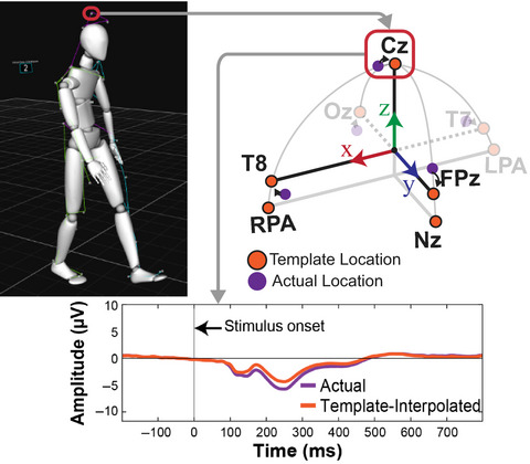
EEG data were recorded from 157 active electrodes with a sampling rate of 1,000 Hz and band-pass filtered from 0.016 to 500 Hz (BrainAmp Move System, Brain Products, Gilching, Germany). Using an elastic cap with an equidistant design (EASYCAP, Herrsching, Germany), 129 electrodes were placed on the scalp, and 28 electrodes were placed around the neck using a custom neckband (EASYCAP, Herrsching, Germany) in order to record neck muscle activity. Data were referenced to an electrode located closest to the standard position FCz. Impedances were kept below 10 kΩ for standard locations on the scalp, and below 50 kΩ for the neckband. Electrode locations were digitized using an optical tracking system (Polaris Vicra, NDI, Waterloo, ON, Canada). Motion capture and EEG samples were recorded and synchronized using labstreaminglayer (https://github.com/sccn/labstreaminglayer).

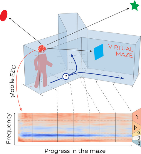
2.3 The invisible maze task

Upon collision of the right hand with an invisible wall, a white disc was displayed 30 cm behind the collision point parallel to the invisible wall much like the beam from a torch in a cave, see Figure 1c. No other visual stimulation was presented inside VR. We did not track the left hand and instructed participants to keep the left arm close to their body. Prior to the first trial, participants were familiarized with the VR scene. To this end, participants were placed in front of a virtual wall and were guided through experiencing the full interactivity of the scene, that is, touching and drawing. When a satisfactory understanding of the interaction possibilities was apparent, participants were asked to take a couple of steps along the wall while touching it to their right-hand side to train the desired task behavior.

(a) Participant displayed from a bird's eye view located at the starting point of an “I”-maze. The star marks the starting position but was not visible during the experiment. Participants were instructed to explore the maze and return to the start after full exploration of the maze. (b) Four mazes were used in the study including an “I,” “L,” “Z,” and “U” shaped maze clockwise from lower left to lower right. Each maze was explored three times before the next maze was learned. (c) Exemplary visual feedback in first-person view in binocular “VR optics” of subject in A (above) touching the wall to the right. No other visual stimulation was presented inside VR. This figure is in part licensed CC-BY and available in color on Figshare (Gehrke et al., 2018)

Performing the task, participants explored four different mazes in the order, “I,” “L,” “Z,” and “U” in three consecutive trials for each maze (see Figure 1b). For each maze, the procedure was as follows: participants were briefly disoriented and then positioned facing the open side of the path. Then, participants were directed to explore the invisible path until they reached a dead end, and subsequently find their way back to the starting position. At the end of each maze and trial, termed “maze trial,” participants received a gamified feedback and were then asked to draw a sketch map of the maze from a bird's eye view. Therefore, participants remained inside VR and an experimenter entered the lab space and handed the participant a computer mouse to control the drawing application. Participants were instructed to start drawing by clicking once with the left mouse button. A red sphere appeared in the VR goggles at the tracked position of the right hand holding the mouse. Holding down the left mouse button, participants were able to draw a red line by moving their hand in space (see Figure 1d). Finally, participants were instructed to take a camera screenshot of their drawing by pressing down the mouse wheel once and holding their final drawing in view. Participants were allowed to erase their drawing and restart at any time by pressing the right mouse button.

The whole procedure was repeated three times in a row for each maze to foster spatial learning within each maze. Between mazes, participants had the opportunity to take a brief break and were made aware of the change to a new maze. The complete experiment, including preparation of physiological measures (electroencephalogram, EEG), took approximately 4 hr. Preceding and following the task, participants completed a set of questionnaires. In this paper, we report how perspective-taking ability as well as self-ascribed sense of direction impacted drawing of sketch maps. In the Perspective Taking and Spatial Orientation Test (PTSOT), participants viewed an array of objects on a sheet of paper and by taking the perspective of one of the objects judged the angle between two other objects in the array (Hegarty, 2002). We recorded the absolute deviation from the correct angle to investigate the impact of perspective-taking ability. The Santa Barbara Sense of Direction Scale (Freiburg Version), FSBSOD, measures self-ascribed navigational ability (Kozhevnikov & Hegarty, 2001). We took the average of all items as the final measure.

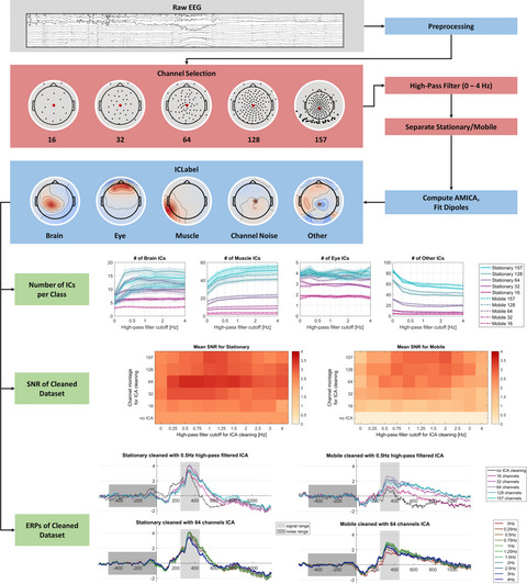
2.4 EEG preprocessing, independent component analysis, and motion capture preprocessing

Electroencephalography data preprocessing and independent component analysis (ICA) were performed with MATLAB 2017a and 2019b (MATLAB, The MathWorks Inc., Natick, MA, USA), using the EEGLAB toolbox (Delorme & Makeig, 2004) and the custom “BeMoBIL Pipeline” scripts and functions. 1 The single subject data were low-pass filtered with 124 Hz and subsequently downsampled to 250 Hz. An average of 12.7 (SD = 2.8) noisy channels were identified and removed through manual inspection on the time domain. Rejected channels were then interpolated while ignoring the EOG channel, and finally re-referenced to average reference (data A). The data were then filtered with a 1 Hz high-pass filter (data B) and a first single-model adaptive mixture independent component analysis (AMICA) (Palmer et al., 2011) was used to identify eye-related independent components (ICs), which were projected out of the sensor data. For this, the rank was reduced by one for the use of an average reference and further by the number of interpolated channels in the respective dataset. To identify eye components, ICLabel (Pion-Tonachini et al., 2019) was used, with components exceeding a value of 0.5 for the “eye” class being defined as eye components. Then, to detect segments of noisy data across channels, an automated time domain cleaning (see Gramann et al., 2018) was performed on narrowly filtered data (data B) from 1 to 40 Hz. The data were therefore first split into 1-s-long segments for which the mean absolute amplitude and standard deviation of all channels as well as the Mahalanobis distance of all channel mean amplitudes were calculated. Results of all three methods were then joined together in order to rank all segments. The 12% highest ranking noisy segments were selected for rejection and an additional buffer of ±0.49 s was added around each segment resulting in about 15% rejected data for each subject. These data were rejected from data B and a second single-model AMICA was calculated on this time domain cleaned data. A dipole fitting procedure was performed for each spatial filter using the 10–20 standard electrode locations and a boundary element head model (BEM) based on the MNI brain (Montreal Neurological Institute, MNI, Montreal, QC, Canada) using dipfit routines (Oostenveld & Oostendorp, 2002). The spatial filter information and equivalent dipole models were then copied back to the preprocessed, interpolated, and average-referenced dataset (data A). Ultimately, all ICs with a “brain” probability smaller than 0.5 as indicated by ICLabel were projected out of the data resulting in the final dataset of likely brain sources and their projections to the channels investigated in all subsequent analyses. Across the study set, 213 ICs were retained forming a sample of 7.3 (SD = 3.8) components per participant. Motion capture data were filtered with a 6 Hz zero-lag low-pass FIR filter and upsampled to match EEG frequency using MobiLAB routines for concurrent analyses (Ojeda et al., 2014).

2.5 Clustering independent components for group-level analyses

To allow for group-level analyses across ICs, we clustered components based exclusively on their equivalent dipole locations, avoiding circular inference (Kriegeskorte et al., 2010). To this end, we employed our region of interest (ROI)-driven repetitive k-means clustering approach (Gramann et al., 2018). ICs were clustered by applying the k-means algorithm with k equal 10 for 10,000 times. ICs with a distance of more than three standard deviations from any final centroid mean were considered outliers. Similar to Gramann et al. (2018), we set the target clustering location to [0, −45, 30] in MNI space. From each of the 10,000 solutions, the cluster with a centroid closest to the target location was selected. Subsequently, the 10,000 selected clusters were ranked via weighting of the cluster's parameter. After applying desirable weights (number of participants: 3, ICs/participants: −2, spread: −1, RV: −1, distance from ROI: −2, Mahalanobis distance from the median: −1), the final clustering solution contained 30 ICs from 22 participants, that is a ratio of 1.3 ICs per participant and a mean RV of 7.9%. Following the assumptions of our clustering approach, which finds an optimal cluster for the given weights, we chose to average IC activity of participants exhibiting more than one IC in the optimized cluster wherever applicable.

2.6 Analyses and statistics

Prior to the statistical analysis, the data were further pruned. The objective was to keep trials comparable across trials and participants. Trials of maze exploration with more than 10 wall collisions were rejected as such exploration behaviors likely reflected participants being stuck “outside” of the maze and not finding their way back into the maze on their own. The number of such trials was very low (six of a total of 348 maze explorations from 29 subjects exploring four mazes three times each). We further rejected four individual explorations because of technical issues (empty battery of the LED driver or loose LED cable). Central for a comparison of trials in which participants were able to build a spatial representation of the entire maze, we further deemed all explorations incomplete where the path was not fully explored as such trials indicated that participants turned around before reaching the dead end and could not build an adequate spatial representation of the maze. With this criterion, 26 explorations were rejected. Overall, 312 maze explorations remained, amounting to 89.7% of the total number of explorations.

2.7 Behavior: Grand averages of sketch map, time-on-task, and number of touches 2.7.1 Sketch map

Two independent raters judged each sketch map drawing. The raters were presented with the question: “Imagine that you can take the present sketch map with you into the virtual environment and use it as a navigational aid. How useful would the map be for you?” To give their rating between 0 (= no help at all) and 6 (= very helpful), they were given the correct shape of the maze to be rated, see for example Figure 1b top left “L” shape, side by side with the drawing to rate, see exemplary “L” sketch maps in Figure 2b. To test inter-rater reliability, we computed Cohen's Kappa with squared weights to emphasize larger rating differences using RStudio Version 1.2.5001 (RStudio Team, 2019; RStudio, Inc., Boston, MA, USA) and package irr (Cohen, 1960; Gamer et al., 2010).

(a) Participants wore high-density wireless EEG, head-mounted virtual reality goggles, and LEDs for motion capture attached to the hands, goggles, and torso. (b) Screenshot of drawn sketch maps of maze L. Three map drawing examples ranging from good (left, rating 6), to intermediate (middle map rating 3), to bad (right, rating 1)

2.7.2 Time-on-task, number of touches, and velocity

Using motion capture, we extracted the time elapsed between the start of each maze trial and the return to the starting position as well as the total number of wall touches during that time window. Reported velocity refers to the magnitude in 2D (ground plane) of the head rigid body. When considering maze complexity, we refer to the number of turns afforded by a maze.

Due to unbalanced data after cleaning with respect to the factorial design, group-level statistics of behavioral data were performed using linear mixed effects model with package lmerTest (Kuznetsova et al., 2017). For each measure: sketch map, time-on-task and number of touches, a linear mixed effects model with fixed effects for Maze and Trial, their interaction and the random effect of participant was fit. Post-hoc contrasts were computed using package emmeans with Tukey's correction for multiple comparisons (Lenth et al., 2020).

2.8 Behavior: Mapping head location at wall touches

To increase the resolution of the exploration behavior, we constructed 2D “bird's-eye view maps” indicating where participants were located when touching a wall. Therefore, for each maze and trial, a 2D histogram with fixed edges, in order to maintain equal resolution across participants, was computed using the (x, y) head location at the times of the wall touches. To increase overlap across participants, a 2D (square sized) Gaussian blur was applied to the resulting histogram image. A σ of 2 was chosen for the 2D filter kernel as it resulted in a good overlap across participants while maintaining spatial specificity. Group-level statistics on the images were performed using MATLAB functions fitrm and ranova. The analysis was conducted for each maze independently due to the shape differences of the mazes. For each pixel, a 1 × 3 repeated-measures ANOVA was conducted across the three trials within subjects. At each pixel, we removed all missing data (see description of the cleaning procedure above) and only conducted model-fitting if data from more than 12 participants were available. Else, the pixel was set to NaN. We corrected for multiple comparisons using false discovery rate (Benjamini & Hochberg, 1995) at α = 0.05. We report both corrected and uncorrected significance masks due to the exploratory nature of the study. To report results, we extracted the F statistic and post-hoc contrasts at a given pixel of interest. For visualization purposes, we removed all patches including less than 2 significant pixels.

2.9 EEG: Spectral maps

To address whether spectral activity of clusters of independent EEG components exhibited spatial specificity during maze exploration, images of spectral activity were constructed at each location (x, y). Therefore, we first computed the power spectral density for moving windows of 1 s length with a step size of 0.2 s between the start and end of each trial using EEGLAB's spectopo function. For computational purposes, we subsequently subsampled motion capture and power data at 1 Hz. In case a subject exhibited more than one IC in the cluster, the power values were averaged across participants. As above, a 2D histogram of the motion capture data with fixed edges per maze was constructed and for each histogram bin, power data were averaged and blurred with a Gaussian with a σ of 2 to increase overlap across participants. Subsequently, maps of individual frequencies (theta 4–8 Hz and alpha 8–13 Hz), trials, and mazes were normalized dividing each map by its mean and subsequently transforming the image values to logarithmic scaling (dB = 10 × log10(power)). Group-level statistics were performed in identical fashion to the head location maps. For plotting purposes, grand averages were first obtained in power and subsequently baseline corrected and transformed to logarithmic scaling.

2.10 EEG: Event-related spectral perturbations at wall touches

For each IC present in the cluster of interest, data were epoched −1 to +3 s around the wall touch event. First, epochs were rejected if the touch duration was longer than 2 s, that is, resulting in a warning signal appearing in the VR where the disc turned red, see Gehrke et al. (2018) for details. The remaining epochs were subjected to a cleaning routine identifying considerable artifacts in the IC activation time course based on epoch mean, standard deviation, and Mahalanobis distance (Gramann et al., 2018). Per participant, the worst 10% epochs were flagged for removal. On average, 723 (SD = 334) epochs remained for further analysis. Time-frequency decomposition was computed via the newtimef function in EEGLAB for 3–80 Hz in logarithmic scale, using a wavelet transformation with three cycles for the lowest frequency and a linear increase with frequency of 0.5 cycles. As participants' behavior was not restricted, wall touches could be of different duration. Therefore, we calculated time-warp anchors across all touches (mean touch duration = 700 ms) and ERSPs were linearly warped to the touch onset (0), the end of the touch (700 ms), and 700 ms succeeding the end of the touch (1,400 ms). Subsequently, phase was discarded, and power values were kept for further analysis. To obtain baseline power spectral density vectors, power values preceding touch events (from −400 to −100 ms) were averaged across time. In case a subject exhibited more than one IC in the cluster, the ERSPs were averaged.

2.11 EEG: ERSP condition average statistics

Statistics on the grand-average ERSP were computed using statconds permutation t-test with 1,000 permutations. For each participant, averaged epochs as well as baseline power were aggregated. Next, the baseline vector was repeated to match the epoch size in time. Permuting epochs and baseline for 1,000 times and computing t-tests result in the distribution under the null hypothesis. To assess statistical significance, the true result was thresholded at α = 0.05 against the null distribution. We corrected for multiple comparisons using false discovery rate (Benjamini & Hochberg, 1995) at α = 0.05. For grand average plotting, participant power averages were aggregated (mean) and subsequently, data of the grand average touch epoch were divided by the baseline vector and the outcome was transformed to logarithmic scaling (dB = 10 × log10(power)). Final plots contain the significance thresholds as contours of significant time-frequency bins. For plotting purposes, significant patches exhibiting less than 50 pixels were removed and the significance mask was filtered using a Gaussian with σ = 1.5.

Group-level statistics for maze, trial, and their interaction were performed using robust repeated-measures ANOVA as implemented in LIMO EEG (Pernet et al., 2011). First, data from one participant were removed due to missing data. Then, epoch as well as baseline power were aggregated (mean) for each maze and trial. Subsequently, power data of the touch epochs were divided by the baseline vectors and the outcome was transformed to logarithmic scaling (dB = 10 × log10(power)). To assess effects, family-wise error rate (FWER) was controlled using threshold-free cluster enhancement (TFCE) as implemented in LIMO EEG. Due to the small sample size (N = 21), only bootstraps containing more than 70% of subjects were considered for the max-TFCE distribution (Pernet et al., 2015). The threshold was set at α = 0.05 of a max-TFCE distribution of 600 bootstraps. As before, we report both uncorrected as well as corrected p-values. For plotting purposes, significant patches exhibiting less than 10 pixels were removed.

2.12 Post-hoc EEG: ERSP single-trial analysis

Following up our analysis on condition averages, we considered the information present in the head location maps and derived the following single-trial analysis scheme. We considered the distance participants traveled between touches in combination with the encounter of a new versus an old wall as efficiently separating the touching behavior in corners versus along straight segments. There, we first computed the distance traveled since the previous successful touch, the Euclidean norm between two succeeding touches. To obtain per participant summaries of ERSP, mass-univariate multiple regression was computed. A linear model was estimated at each time-frequency pixel. The linear model was defined as tf_pixels = intercept + distance_traveled × wall_change + baseline. In order to estimate the interaction term, both predictors were z-scored prior to model fitting. To further infer whether components of the event-related response could be explained by baseline activity, baseline power was entered as a predictor. To assess effects, statconds one-sample permutation t-test with 1,000 permutations were computed using the betas per participant. Subsequently, the surrogate t-tests were transformed to the TFCE statistic (Pernet et al., 2015). The threshold for multiple comparison was set at α = 0.05 of the max-TFCE distribution of 1,000 permutations. For plotting purposes, significant patches exhibiting less than 10 pixels were removed.

3 RESULTS 3.1 Behavior

The sketch map usefulness ratings revealed a very high agreement between the two raters' judgments, Cohen's κ = 0.835, p < 0.001. Participants drew useful sketch maps already after the first maze trial (intercept: t124.5 = 9, p < 0.001; see Figure 2 for exemplary sketch maps and their average usefulness rating). On average, 2/3 were able to draw very useful sketch map, see Figure 7, with the remaining third exhibiting an average sketch map rating of less than 2, referring to a sketch map that is of little help as a navigational aid. With repeated maze explorations, ratings of the usefulness of the drawn sketch maps did not further improve (F2,271.3 = 1.8, p = 0.16, mean first 3.2, SD = 2.1, second 3.6, SD = 1.9, and third trial 3.7, SD = 1.9), nor did they vary as a function of maze complexity (F3,272.25 = 1, p = 0.4, mean “I” 3.6, SD = 2.1, “L” 3.7, SD = 1.8, “Z” 3.3, SD = 2.1, and “U” 3.3, SD = 1.9) and their interaction. We confirmed that individual differences in spatial ability had an impact on the sketch map drawings. Increasing perspective-taking and spatial orientation ability, as assessed with the PTSOT questionnaire, positively impacted the rating of sketch maps (b = 0.02, F1,27 = 4.9, p = 0.036, R2 = 0.15). We observed no impact of the subjective Santa Barbara Sense of Direction Scale on sketch map quality. As previously reported in Gehrke et al. (2018), we observed a decrease in time-on-task with repeated explorations (F2,271.8 = 17.6, p < 0.001) and a main effect of maze complexity, operationalized by the number of turns in the maze. More specifically, time-on-task decreased significantly comparing the first and second (t272 = 4.47, p < 0.001), as well as the first and third trials (t272 = 5.57, p < 0.001; see Figure 3a). The number of wall touches decreased with repeated explorations (F2,271.1 = 26.1, p < 0.001) with a significant decrease from first to second (t271 = 4.63, p < 0.001), first to third (t272 = 7.01, p < 0.001) as well as second to third (t272 = 2.4, p = 0.045) trial (see Figure 3b). Furthermore, participants moved faster with increasing explorations (F2,272.35 = 46.1, p < 0.001; see Figure 3c), as well as in simple compared to more complex mazes (F2,274.1 = 6.8, p < 0.001). However, no interaction effect was observed. The main effect of maze complexity on velocity was driven by the “I” maze, with significant linear contrasts between the “I” maze and all other mazes, for example, “I” – “U” (t276 = 4.23, p < 0.001).

Top row: Box-Whisker plots with individual observations of each participant averaged across maze configurations for each repeated maze trials 1–3. (a) Duration in seconds elapsed between the start and end of each exploration phase, (b) Number of wall touches during the exploration phase, and (c) Movement Velocity in meters per second. (d) 2D histograms of the head location at wall touch moments for all three explorations in each maze “I,” “L,” “Z,” and “U.” Warmer colors indicate more wall touches/time spent at location. Solid (corrected) and dotted (uncorrected) contours mark significant pixels of repeated explorations

To further investigate participants' exploration behavior, head locations were mapped at moments of wall touches indicating that participants sampled corners and dead ends more frequently than straight segments (see warmer colors in Figure 3d). Specifically, at the dead-end of the “I” maze (F2,28 = 6.1, p = 0.005 uncorrected) and “U” maze (F2,28 = 18.9, p < 0.001, FDR corrected), a decrease in the number of touches was observed as a main effect of trial. Furthermore, a change in touch frequency was observed at the inside turn in the “L” maze (F2,28 = 5.6, p = 0.001 uncorrected), trending down from earlier to later trials.

Taken together, participants took less time exploring the mazes in repeated explorations, needed fewer wall touches, and moved faster, Figure 3a–c. In detail, we observed participants spending most of their time exploring “outside” (convex) corners and in the dead ends, Figure 3d. This exploration pattern was largely unaffected by repeated explorations.

3.2 Oscillations of independent EEG sources located in or near retrosplenial complex

Clustering ICs resulted in a cluster with a centroid location around X = 3, Y = −52, Z = 24 (MNI), a mean residual variance of 7%, containing 22 of 29 participants and 30 ICs, see Figure 4a. The MNI coordinates refer to the posterior cingulate bordering on the precuneus in the AAL atlas and BA23 (posterior cingulate cortex) in the Brodmann atlas, respectively.

(a) Locations of equivalent dipole models projected onto a standard brain space (MNI) with each small sphere representing individual ICs and the bigger sphere representing the cluster centroid. The cluster centroid was located in retrosplenial complex (x = 3; y = −52; z = 24), containing 30 ICs from 22 participants (corresponding to 74% of all participants). (b) Images of theta (4–7 Hz, top) and alpha (8–12 Hz, bottom) power for all three explorations in each maze “I,” “L,” “Z,” and “U.” Warmer colors indicate higher power. Solid (corrected) and dotted (uncorrected) contours mark significant pixels of repeated explorations

Mapping continuous spectra to spatial locations revealed a main effect of repeated maze trials on theta band activity at the dead end of maze “I” (F2,42 = 12.3, p < 0.001), see Figure 4b top left, with the first trial exhibiting a higher power increase over its baseline then the subsequent trials two and three. Similarly, at the dead end of maze “I,” alpha power was affected by repeated maze trials (F2,42 = 13, p < 0.001), see Figure 4b bottom left. Further patches of a main effect of repeated explorations were observed for maze “I” at the center of the maze path as well as toward the left wall (left from the starting position) in both theta and alpha frequency bands. For the other mazes, repeated explorations did not impact continuous theta nor alpha spectral power following correction for multiple comparison. Not correcting for multiple comparisons, mazes “L,” “Z,” and “U” exhibit slight effects of maze trial at the first turn segments (“L” and “U”) as well as at the second turn (“Z”) in the theta frequency band, see Figure 4b top. Overall, visual inspection hints at a concentration of power increase over the full-trial baseline at corners and dead ends in later compared to earlier trials and more so in theta than alpha frequency (see for example Figure 4b top “Z” and “U” mazes).