1 Introduction

Alzheimer's disease (AD) is a severe neurological condition. A person with AD is unable to converse, retain details, make decisions, pick up new skills, and so on (Korolev, 2014; Hazarika et al., 2023). The majority of people with Alzheimer's disease are elderly or in their early 60s. The most catastrophic of all the physical alterations is damage to brain cells. The brain areas that sustain the most significant damage are the amygdala, hippocampus, and a few additional areas that control most AD symptoms. The patient is unable to perform even the most basic tasks because learning cells are first impacted, then additional gray matter cells are destroyed. Consequently, those suffering from Alzheimer's disease experience extreme behavioral and cognitive challenges in addition to memory loss. The majority of individuals with AD have advanced from Mild Cognitive Impairment (MCI), an early stage of dementia. The symptoms of MCI are nearly the same as those of AD, albeit less severe. MCI is sometimes called AD in its early stages. Research indicates that eight out of ten individuals with MCI acquire AD within 7 years (Hazarika et al., 2023). Typically, neuro-specialists work alongside psychologists to administer various mental and physical examinations, including a Mini-Mental State Examination (MMSE), a neurophysiological assessment, a physical assessment and screening tests, a depression analysis, and more. Various instruments are needed to complete these tasks, making the procedure inefficient and time-consuming. To provide tissue-by-tissue information on the neurological system, Magnetic Resonance Imaging (MRI) is a widely used method. Compared to the conventional diagnosis method, brain imaging may require less time and equipment for AD classification. Furthermore, proper brain imaging processing may identify significant biomarkers long before the beginning of Alzheimer's disease (Hazarika et al., 2023). Conversely, intricate pixel formations make diagnosing AD difficult by looking at tissue changes for traditional image processing methods (Fung et al., 2019). Sample brain MRI scans for patients with AD, MCI, and Cognitively Normal (CN) are shown in Figure 1.

Figure 1. Sagittal middle slice of (A) Alzheimer's disease (AD), (B) Mild cognitive impairment (MCI), (C) Cognitively normal (CN).

The intricacy of Alzheimer's disease and the necessity of timely identification make it a formidable medical issue. Conventional techniques might not always be enough to predict the course of the illness with enough accuracy. Alzheimer's is a complicated medical condition that requires prompt diagnosis due to its complexity. Deep Learning (DL) techniques are increasingly being used by medical experts to visualize and predict diseases and create individualized, preemptive treatment regimens (Saleh et al., 2023). Traditional Machine Learning (ML) and DL algorithms aimed to solve discrete, highly data-intensive jobs. Transfer learning has emerged as a solution to the isolated learning paradigm to improve classification performance using MRI scans. Its goal is to use the characteristics learned from pre-trained models. Creating effective models to help radiologists and medical professionals recognize the various phases of Alzheimer's disease, such as AD, MCI, and CN.

Francis et al. (2024) employed a deep learning model to evaluate the ADNI dataset and identify the stages of Alzheimer's disease using Squeeze and Excitation Networks (SENet) and local binary patterns. The accuracy of classifying MCIc (MCI converter) against MCInc (MCI non-converter) was 86% with SE networks and 82% without SE networks. Lu et al. (2022) developed a two-stage model that used contrastive learning and transfer learning (ResNet) to predict the progression of MCI into AD, with an accuracy of 82% and an AUC of 84%. The improvised model ADNet was created by integrating SENet to VGG-16 and improving feature extraction after evaluating the ADNI 2D MRI images. Without SENet, the accuracy in AD vs. CN classification was 82.94%, but with SENet, it was 84.08%. By developing an optimal weighted ensemble model consisting of five pre-trained 3D CNN ResNet-50 variants (ResNet, ResNeXt, SEResNet, SEResNeXt, and SE-Net), Dharwada et al. (2024) concentrated on early AD diagnosis using sMRI images from the ADNI dataset and achieved an accuracy of 97.27%. Illakiya et al. (2023) developed a hybrid attention model to extract both global and local features by utilizing 3D MRI from ADNI. It achieved an accuracy of 89.17% with DenseNet-169 along with SENet. With DenseNet-169 alone, able to reach 77% accuracy. Khan et al. (2022) suggested PMCAD-Net, an applicable multiclass classification network for the early detection of Alzheimer's disease. Using the ADNI dataset, it distinguishes between EMCI, LMCI, CN, and AD, achieving a 98.9% accuracy rate and a 96.3% F1 score. Khan et al. (2023) proposed a transfer learning-based method (VGG-16 and VGG-19) that differentiated between CN, EMCI, LMCI, and AD by using tissue segmentation to extract gray matter from the ADNI dataset's MRI images and achieved an accuracy of 97.89%.

Odusami et al. (2021) was able to analyze fMRI images from ADNI and predict the early stages of AD with an accuracy of 80.80% for AD vs. CN categorization by unfreezing all layers of ResNet-18 and modifying all parameters to fit the new dataset. The accuracy of the ensemble model developed from the analysis of fMRI images from ADNI was 97.9%, 87.5% with ResNet-18, and 96.2% with VGG-16 in Tajammal et al. (2023). Utilizing an attention mechanism, ResNet-18, Zhou et al. (2023) developed a 2D parameterized model. While average pooling produces an accuracy of 88.12%, ResNet-18 alone produces an accuracy of 82.45%. A ROC of 98.49% is provided by the complete model. Suja and Raajan (2024) evaluated a number of deep learning models for the timely diagnosis of AD using the ADNI dataset. The accuracy of the ResNet-18 model with RMSprop and ADAM was 83.5%. Topsakal and Lenkala (2024) proposed an ensemble model that used a pre-trained, improved model with gradient boosting to attain a 95% accuracy rate. However, ResNet-50 alone had an accuracy of 88%.

However, graph convolutional networks can analyze the pathological brain regions associated with cognitive disorders and achieve good classification performance. They cannot uncover the fundamental relationships between multiple brain ROIs associated with illness. These networks first retrieve characteristics for each ROI or subject before building a classifier for AD diagnosis using either unimodal or bimodal imaging data. Utilizing hypergraph-based techniques, which consider high-order relations between numerous ROIs from unimodal or multimodal imaging, improved classification performance and created discriminative connections.

Zuo et al. (2024) designed a Graph-based model and forecast aberrant brain connections at various AD stages. The prior distribution from graph data is estimated using a Kernel Density Estimation (KDE) technique, and an adversarial learning network is integrated for multimodal representation learning. The Pairwise Collaborative Discriminator (PCD) preserves sample and distribution consistency, and a hypergraph-based network is developed to fuse the learned representations to produce united connectivity-based features. For the binary classification (AD vs. CN, LMCI vs. CN, and EMCI vs. CN), 300 individuals were gathered from the ADNI-3 database for the investigation. The accuracy rates were 96.47%, 92.20%, and 87.50%, respectively. Pan et al. (2024) developed a comprehensive system integrating fMRI and DTI to identify aberrant brain networks for AD research. This study used 236 ADNI subjects and obtained an accuracy of 80.72% for CN, 63.8% for EMCI, 86.91% for LMCI, and 82.71% for AD. Zong et al. (2024) constructed brain networks using Diffusion-based Graph Contrastive Learning (DGCL) to identify the geographical positions of brain regions precisely. Contrastive learning is adopted to optimize brain connections by removing individual differences in redundant connections unrelated to disorders. Data (DTI format) from 349 subjects-including those in the Control Normal group (CN), Early Mild Cognitive Impairment (EMCI), Late Mild Cognitive Impairment (LMCI), and AD were gathered from the ADNI, and an accuracy of 86.61% was produced. Zuo et al. (2023) presented a brain structure-function fusing learning model by fusing representation from rs-fMRI and DTI to investigate MCI. The knowledge-aware transformer module automatically captures features of local and global connections across the brain. Achieved an accuracy of 87.80% for EMCI vs. Subjective Memory Complaints (SMC), 95.57% for LMCI vs. SMC, and 91.14% for LMCI vs. EMCI.

Every deep learning network that is constructed from the ground up will run into a lot of issues. A Deep CNN network requires a large number of parameters to be trained during the training phase. By lowering this parameters, the network's computational complexity and time and space constraints would decrease. For the same reason, we can use Squeeze and Excitation blocks to minimize the total training parameters, identify the channel interdependencies, and recalibrate the output feature with input to exploit the local and global spatial features to improve the performance. We can also use Depth Convolution instead of standard Convolution. The fully connected layer, including the dropout layer, can be replaced with Global Average Pooling to lower the overall training parameters and accelerate convergence. This regularization technique significantly reduces overfitting and generalization errors in the model. However, an extensive dataset for model training and meticulous hyperparameter optimization for increased efficiency are no longer necessary when employing the Transfer Learning technique. The main contributions of our work are as follows.

• Squeeze and Excitation (SE) blocks were added to the ResNet-18 residual block in order to build a Deep CNN ResNet-18-based model from the ground up using the attention mechanism. Additionally, to lower training parameters and lighten the model overall, we employed Depth-wise Convolution and Global Average pooling. ROC and accuracy were compared to various combinations of optimizers, dropout rates, sample sizes, and epochs using the ADNI dataset, which was utilized to train the model. Cross-validation is used to validate the model and lower the regularization errors.

• The accuracy and ROC were assessed through training and testing using the pre-training model ResNet-18 with SE block and ADNI dataset.

• Through training and testing with the pre-training model ResNet-18 without SE block, the accuracy and ROC were evaluated using the ADNI dataset.

• ROC values, testing and training accuracy, confusion matrix, and other evaluation parameters were used to compare the performance of the three models mentioned above.

• The models were assessed using real-time patient MRI scans along with their demographic data as well as with the OASIS-1 dataset.

Medical professionals are using deep learning for disease prediction and visualization to create personalized treatment plans (Saleh et al., 2023). In comparison to the three deployed models and the state-of-the-art techniques outlined, ResNet-18, a pre-trained model with SE block, demonstrated the most convincing performance.

Five distinct sections that make up the overall paper. An outline of Alzheimer's disease, the motivation behind this effort, and a survey summary of associated works are covered in Section 1. Section 2 describes the dataset, data pre-processing, and proposed model's architectures in detail. The results are demonstrated and compared using several criteria in Section 3. Lastly, the conclusion, limitations, and future work are discussed in Sections 4 and 5.

2 Materials and methods

The initial section outlines the datasets utilized for training and evaluating all the models, along with a detailed description of the preprocessing steps that make these datasets suitable for both training and testing. The following section explains the functionality of the Deep CNN architecture based on ResNet-18, which was developed from scratch. This architecture incorporates depthwise convolution and the Squeeze and Excitation algorithms. Additionally, it reviews the framework of two other models that employ a transfer learning approach. Figure 2 shows the complete procedure of our suggested methodology.

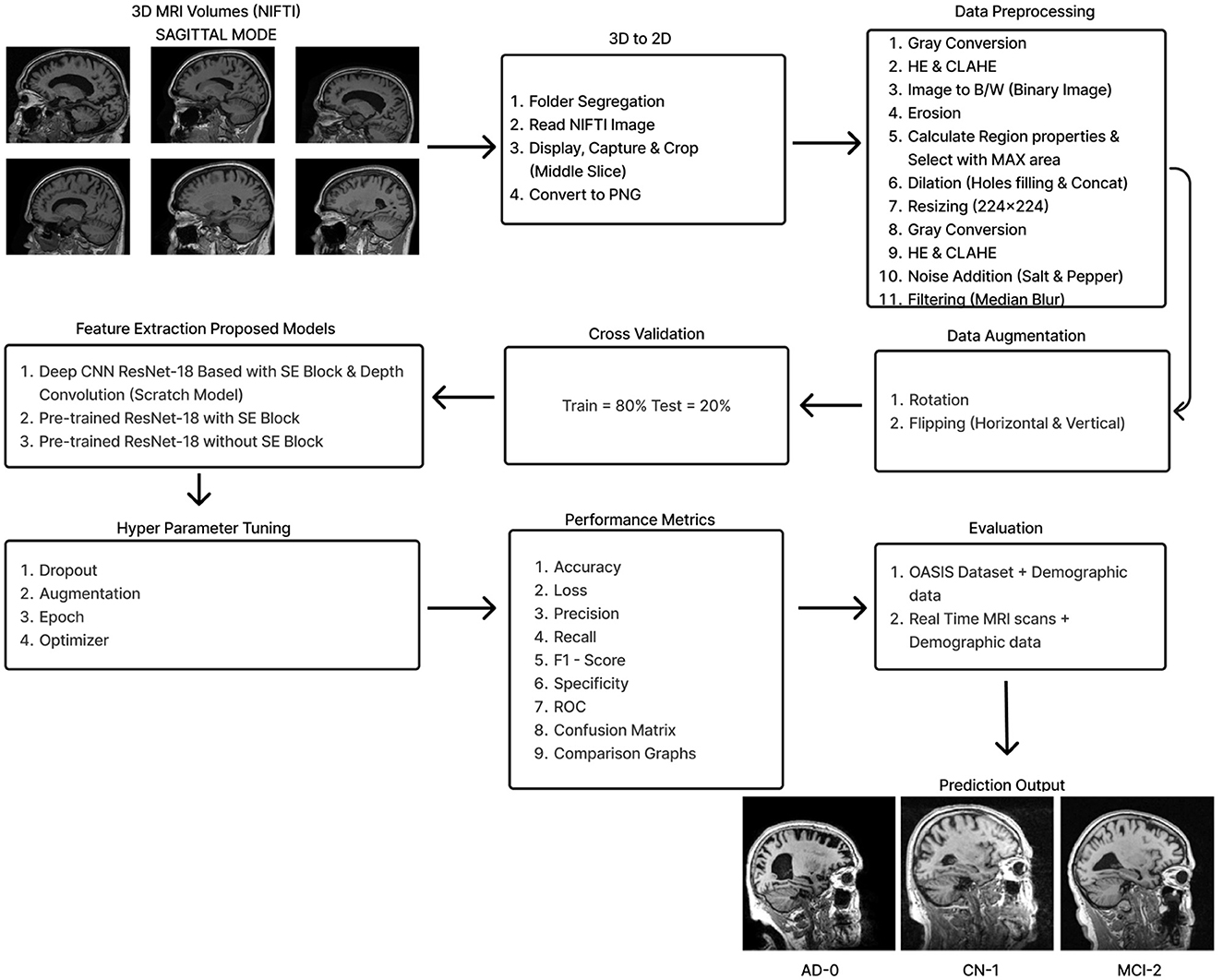
Figure 2. Overall procedure.

2.1 Dataset

This section covers the datasets used for training and testing, along with details about the preprocessing methods applied to 8-bit images available in each dataset.

2.1.1 ADNI

The ADNI (Alzheimer's Disease Neuroimaging Initiative) database (http://adni.loni.usc.edu/ accessed on August 2022) provided the study's data. These comprised the core of our analysis: volumetric T1-weighted, B1 corrected, N3 scaled, Magnetization-Prepared Rapid Gradient Echo (MP-RAGE) MRIs with Gradwarp. Alzheimer's Dementia (AD), Cognitively Normal (CN), and Mild Cognitive Impairment (MCI) were the three categories of the dataset that comprised the 2291 (476-AD, 703-CN, 1112-MCI) patients in this study. It is 46.83 GB compressed and 70.8 GB uncompressed and contains MRI images in NIFTI format. A single NIFTI image contains a packed volume of ~184 slices.

2.1.2 Real-time hospital patient data

MRI imaging data from eight patients at the Government Medical College in Kottayam, Kerala, were collected for model evaluation. Each patient had around 250–400 DICOM images converted to JPG format. From these, six to nine sagittal-mode JPG images were randomly selected for pre-processing. They also provided the manually conducted tests for the MMSE and the CDR, along with their corresponding scores.

2.1.3 OASIS-1

OASIS-1 (Open Access Series of Imaging Studies) is a publicly accessible dataset used to test our approach. It is 15.8 GB compressed and 50 GB uncompressed and available at http://www.oasis-brains.org. Twelve archive files are available for download, organized by imaging session. Each session directory contains an XML file, a TXT file, and three subdirectories: RAW, PROCESSED, and FSL_SEG. The XML and TXT files provide acquisition and anatomical measurements, while the RAW directory holds the individual scan images. The PROCESSED directory includes two subdirectories: SUBJ_111 and T88_111. The SUBJ_111 folder contains averaged and co-registered sagittal images in GIF format. The T88_111 folder has the atlas-registered, gain field-corrected image and its brain-masked version for all three projections, also in GIF format. The FSL_SEG directory contains the segmentation image for gray matter, white matter, and Cerebro Spinal Fluid (CSF) generated from the masked atlas image. The “oasis_cross-sectional.csv” spreadsheet contains labels for demographics, clinical information, and derived anatomic volumes. Ten randomly selected sagittal GIF images were converted to JPG format for applying our various pre-processing algorithms, enabling model testing.

2.1.4 Data preprocessing

All three datasets were mainly preprocessed using MATLAB. For the ADNI dataset, the middle slice was carefully selected to observe the hippocampus region, which is the area most significantly affected by Alzheimer's disease (AD). Initially, the MRI images in NIFTI format were displayed and captured as a 2D image focusing on the middle slice using the screen capture function. The captured image was then cropped and saved in PNG format. Subsequently, the 2D images were organized into three distinct folders labeled AD, CN, and MCI, with assistance from the provided CSV file.

Preprocessing starts by converting the RGB image to grayscale to simplify the data and focus on intensity variations. Histogram Equalization is then applied to enhance contrast by stretching the pixel intensity histogram, improving detail visibility in different lighting conditions. Contrast_Limited_Adaptive Histogram Equalization (CLAHE) is used to boost contrast in low-contrast areas (Khalid et al., 2023). A binary image is created with a threshold of 0.3 to distinguish regions of interest from the background, followed by a few morphological operations to analyze the shapes and structures in the image. Erosion is an operation that reduces the size of an object by removing pixels from its boundaries. It utilizes a flat diamond-shaped structuring element with a distance of 3 units from the origin to the points of the diamond. After performing erosion, region properties are calculated, and the region with the maximum area is selected. Following this, morphological dilation is applied to restore the eroded regions and enhance the prominent features. The dilation uses a flat diamond-shaped structuring element with a distance of 8 units, as well as a disk-shaped element with a radius of 5 units. After dilation, morphological hole filling is used to address any gaps or holes within the segmented region. This process ensures that the area is complete and contiguous. As a result, the techniques applied yield a segmented image that clearly highlights the specific location of the disease within the Alzheimer's images, providing a precise visualization for further analysis.

The segmented image is resized to 224 × 224 pixels to ensure uniformity across the datasets, which facilitates efficient training. Subsequently, gray conversion, histogram equalization, and CLAHE are applied to simplify the data and further enhance image contrast. An impulsive noise, known as Salt-and-Pepper, is then introduced to the image to evaluate the robustness and effectiveness of the filtering technique. Finally, a compatible non-linear Median Blur filter technique is employed to remove the impulsive noise while preserving essential image details effectively.

During the preprocessing of the ADNI dataset, the following times were recorded for a single image:

• AD image: 0.9456 s for 2D conversion and 4.0455 s for preprocessing, totaling 4.9911 s.

• CN image: 0.9901 s for 2D conversion and 3.3949 s for preprocessing, totaling 4.385 s.

• MCI image: 1.2496 s for 2D conversion and 3.2866 s for preprocessing, totaling 4.5362 s.

The total preprocessing time for a single real-time image was 14.1287 s, while the OASIS-1 image took 12.6313 s. The complete path flow of image preprocessing is shown in Figure 3.

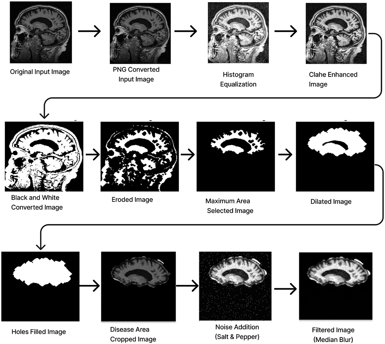
Figure 3. Image pre-processing.

2.1.5 Data augmentation

Although convolutional neural networks offer a great deal of generalization potential, this ability is severely constrained when the data set is small. This is due to the overfitting of the model. The problem of insufficient data could be efficiently addressed by utilizing data augmentation technology, which has been used to enhance the ADNI dataset using digital image processing technology (Gao et al., 2021). Owing to the restricted amount of data, the original dataset is supplemented by flipping horizontally, flipping vertically, and rotating. When an image is rotated, it is oriented around its center at a particular angle. A rotation of –15 to +15 is used in this investigation. The goal is to generate perspective adjustments from the same image so that models trained on more data can adapt better to changes in the orientation of the image's objects (Hasanah et al., 2023).

Data augmentation resulted in an expansion of the dataset from 2,291 images (476-AD, 703-CN, and 1,112-MCI) to 14,760 images (3,067:AD, 4,528:CN, 7,165:MCI) in the first stage and 25,357 images (5,267:AD, 7,779:CN, 12,311:MCI) in the second stage. This could perhaps solve the overfitting problem to some extent. In order to regularize the model and reduce the generalization error, the cross-validation techniques are then applied in an 80:20 ratio.

2.2 Deep CNN ReNet-18 based scratch model

This part will cover the Deep CNN ResNet-18-based model with the SE block and Depth Convolution in detail and explain each embedded block in the architecture.

2.2.1 ResNet-18 pre-training model

ResNet-18 is composed of three layers: 17 convolution layers, a max pooling layer with a 3 × 3 filter size, and a fully connected layer. The block diagram for the pre-training ResNet-18 model is shown in Figure 4A. The ResNet-18 network is based on a residual building component (Gao et al., 2021). Figure 4B shows the structure of the residual building component.

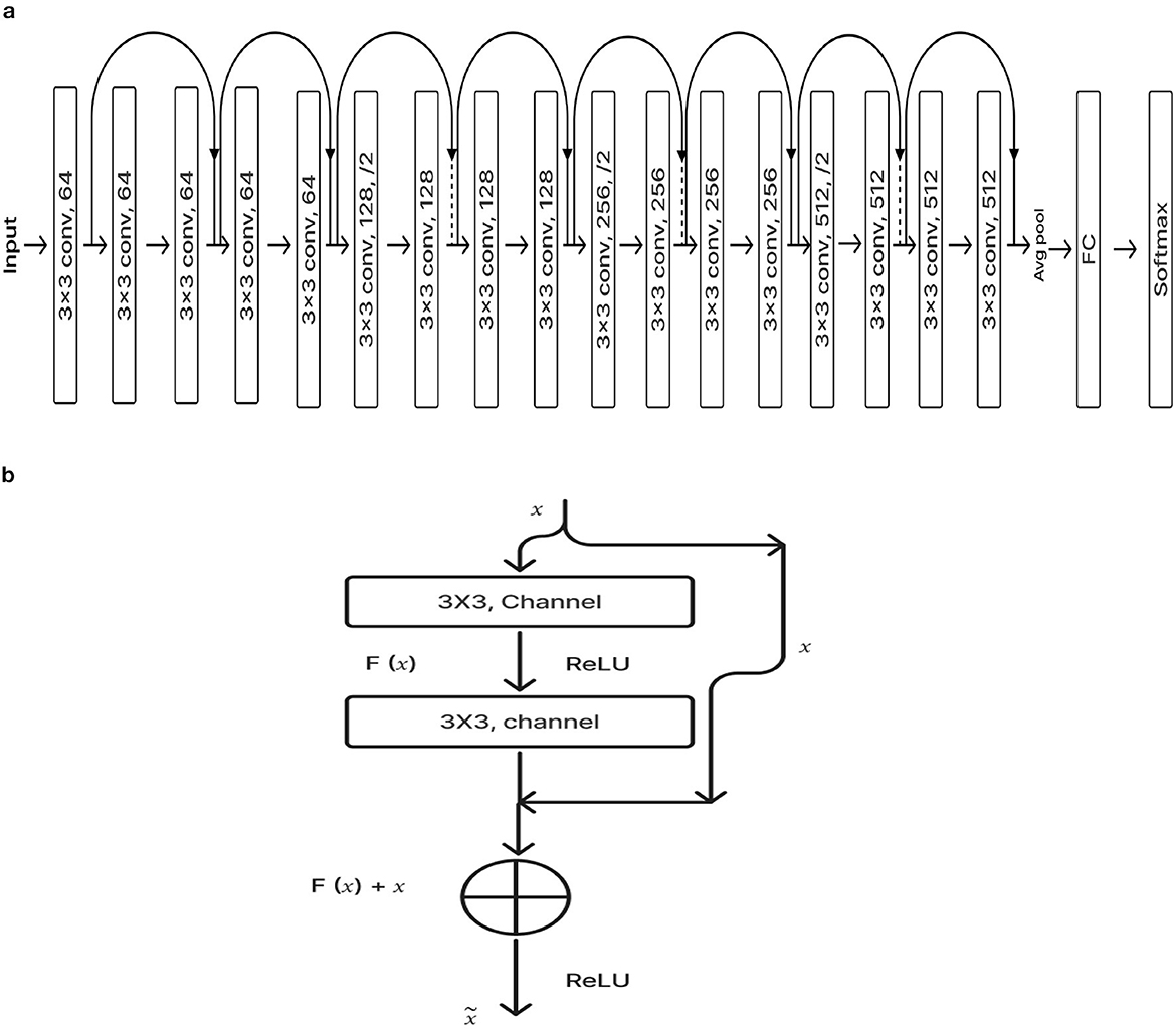
Figure 4. (A) ResNet-18 pre-training model. (B) Residual network.

After adding the input and output vectors directly through the convolutional layer, the result can be produced using the rectified linear unit (ReLU) activation function. This method can effectively address the issue of a deeper neural network's vanishing and exploding gradient. F stands for the residual function, while x and y, respectively, denote the input and output, which are referred to by Equation 1 (Odusami et al., 2021; Gao et al., 2021; Hasanah et al., 2023).

2.2.2 Transfer learning

Transfer learning is a useful technique for training deep learning (DL) models that leverage information from one domain to enhance performance on a different but related task or domain (Saleh et al., 2023). Pre-trained models are trained on large datasets, such as ImageNet, which comprises millions of images with over a thousand labels. As a feature extractor of general features, it is sensible and useful to apply the domain knowledge from these models to other domains, including medical classification tasks (Saleh et al., 2023). Due to the medical nature of the target data, we are unable to utilize the pre-trained model fully. We must address domain-specific difficulties in order to adjust the output layer. Reducing the number of training parameters needed to accomplish a task, increasing accuracy, and saving time are all achieved by using knowledge transfer models rather than randomly started models. This enables effective discrimination between the different classes in the dataset. In order to assist doctors in making precise and fast diagnoses, it first reduces the need for vast volumes of labeled data and offers a comprehensive and precise classification framework. This method solely trains the weights of the recently added layers for the particular task, freezing the weights of the previously trained model before training. This tactic lessens the problems brought on by a small and uneven dataset. The flow chart of our proposed model, which makes use of the Transfer Learning concept (Saleh et al., 2023; Gao et al., 2021), is shown in Figure 5.

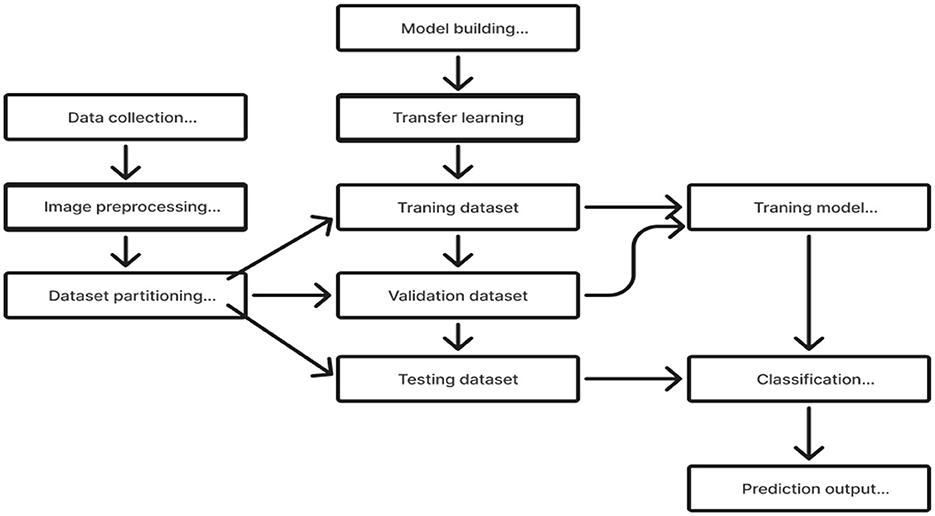
Figure 5. Transfer learning application.

2.2.3 Global average pooling

The fully connected layer is a common classifier used by CNN. Training will be hindered and over-fitting is more likely due to the fully connected layer's excessive amount of parameters. Global average pooling, or GAP, is the procedure that generates the output by taking the global average of all the pixels in the feature map for each channel. These output feature vectors will be sent straight to the classifier, providing each channel with useful information (Gao et al., 2021).

2.2.4 Depth-wise convolution

The model performs more slowly and uses more memory than many other models when convolutional procedures are utilized extensively. We propose to use depth-wise convolution layers rather than standard convolution ones to solve this issue. Depth-wise convolution is a common technique for reducing the parameters and improving computational and representational efficiency. In this procedure, a distinct filter is applied to each input channel, and a point-wise 1 × 1 convolution is used to merge the outputs.

Ĉk,l,a=∑i,jK^i,j,a.Zk+i-1,l+j-1,a    (2)

The depth-wise convolution filter of size PK × PK × X is denoted by K^ in Equation 2, where X is the sum of the input channels and PK is the spatial dimension. Here, the ath channel for the filtered feature map Ĉ is created by using the ath kernel from L^ in the ath-channel of Z.

PK·PK·X·PZ·PZ    (3) PK·PK·X·PZ·PZ+X·Y·PZ·PZ    (4) PK·PK·X·PZ·PZ+X·Y·PZ·PZPK·PK·X·Y·PZ·PZ    (5)

Equation 3 can be used to calculate the depth-wise convolution's computational cost, It is less expensive than the computing cost of the regular convolution operation. Y is the total output channels. A 1 × 1 point convolution is used to merge the depth-wise convolutions. The total cost, including the point convolution, can be written as Equation 4. Equations 5, 6 can express the overall cost reduction (Hazarika et al., 2022b,a).

2.2.5 Squeeze and excitation (SE) block

The global features at the channel level are initially extracted by the SE module using the Squeeze function on the feature map. It then presents the Convolution function. The global features are then subjected to an application of the Excitation function in order to ascertain the weights of each channel and comprehend their interrelation. Multiplying the recently added mapping feature yields the final features.

To build a Squeeze-and-Excitation block, begin with a convolution operation Ftr translating an input X ∈ ℝH′ × W′ × C′ to feature mappings U ∈ ℝH×W×C. We use a collection of learned kernels, V = [v1, v2, ....vC], where vC denotes the parameters of the Cth filter. Show the outputs as U = [u1, u2, ....uC],

uc=vc*X=∑s=1C′vcs*xs    (7)

where “*" is the convolution operation and vcs is a 2D spatial kernel that translates to a single channel of vc on the corresponding channel of X. Channel dependencies are implicitly incorporated in vC as the output is the total of all channels. The filters capture the local spatial correlation (Hu et al., 2018; Yang et al., 2022).

The model's attention mechanism allows it to suppress the less important channel properties and prioritize the more informative ones. This attention mechanism memorizes the spatial correlations between the information after receiving the spatial properties in a channel as input. Under the convolution results of each channel, the sum of the channels has been calculated concurrently, and the spatial relations learned by the convolution kernel can be merged with the relationships between channel characteristics. To fully describe channel-wise dependencies, it has to learn a nonlinear interaction between channels and a mutually exclusive relationship. To meet these needs, we employed a straightforward gating mechanism with Sigmoid activation.

zc=Fsq(uc)=1H×W∑i=1H∑j=1Wuc(i,j),z∈ℝC    (8) s=Fex(z,W)=σ(g(z,W))=σ(W2δ(W1z))    (9)

W and H are the width and height of the mapping features, respectively and W1∈ℝCr×C, W2∈ℝC×Cr

To simplify the model and enhance its capacity for generalization, two fully connected (FC) design layers have been employed. The first FC layer contributes to dimension reduction, and “r" is a parameter for the dimension reduction factor. ReLU activation can then be performed. The last layer of FC adds a new dimension. New features on U can eventually be multiplied by the learning activation levels of each channel. The final output of the block is derived by rescaling U using the activations ‘s":

xc~=Fscale(uc,sc)=scuc    (10)

where X~=[x1~,x2~,....xC~] and Fscale(uc, sc) denote the channel-wise multiplication between the scalar sc and the feature map uc∈ℝH×W. Equation 7 through Equation 10 provide a mathematical representation of the full function (Hu et al., 2018; Gao et al., 2021; Alazwari et al., 2024).

2.2.6 Deep CNN_ResNet-18 based scratch model with SE and depth wise convolution

The proposed Deep CNN model was built on the following principles: Squeeze and Excitation (attention mechanism), Depth convolution, and Residual structure. The proposed architecture is shown in Figure 6. We see the Convolution Block (CB-Block), Identity Block (IB-Block), and Squeeze and Excitation Block (SE-Block) in Figure 7. The following describes this architecture's key components. A Squeeze and Excitation (SE) block is integrated with a Deep CNN model that is based on a ResNet-18 model and was created from scratch using a unique architecture. Moreover, Depth convolution was used instead of regular convolution. The Convolution blocks, Identity blocks, and SE blocks are used in this six-part architecture. This proposed model with SE block consists of two convolution layers (C1 and C2), four convolution blocks (CB1, CB2, CB3, and CB4), four identity blocks (IB1, IB2, IB3, and IB4), SE Block, Global Average Pooling layer, and two Fully Connected layers (FC1 and FC2).

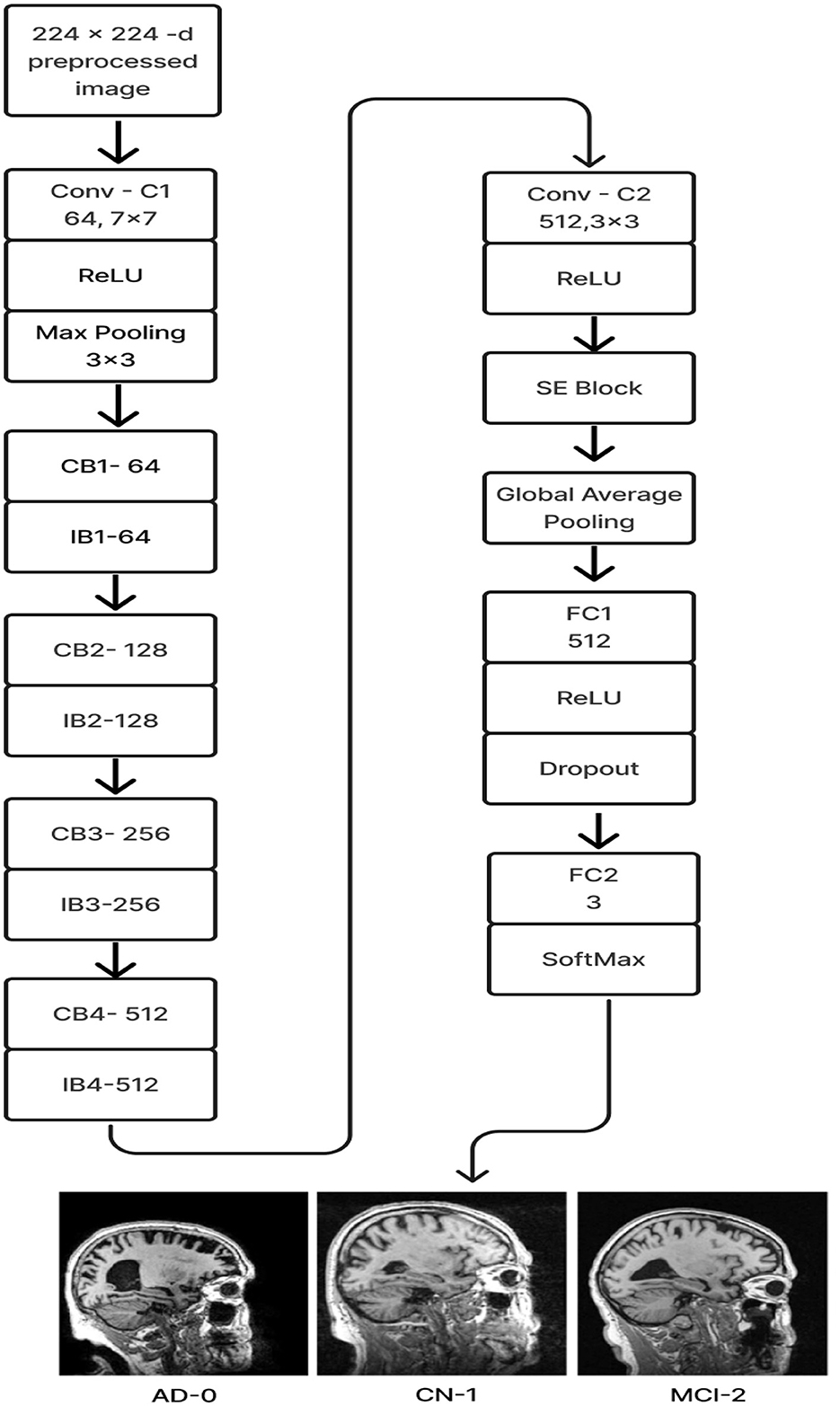
Figure 6. Proposed model 1: deep CNN_ResNet-18 based scratch model with SE and depth convolution.

Figure 7. (A) Convolution block (CB). (B) Identity block (IB). (C) squeeze and excitation block (SE).

Batches of sagittal slices from MRI brain scans with dimensions of 224 × 224 × 1 are accepted as input. A max-pooling layer with a kernel size of 3 × 3, a batch normalization layer, a ReLU activation function, and a convolutional layer with a kernel size of 7 × 7 are employed in the first section, C1. The max-pooling layer preserves important feature information while reducing the model's size and parameters and expanding the receptive fields. Beginning with a depth-wise convolution, the Convolution Block in the second section proceeds with a convolution layer and ReLU activation. Afterward, an Identity Block, which comprises the ResNet-18 model's residual portion, is employed to address the vanishing and exploding gradient issues that most deep-learning networks encounter. The third part, which consists of convolution C2 followed by ReLU activation, receives the combined output of the second part as input. The fourth part, SE-Block, includes the Squeeze-and-Excitation (SE) module.

The SE module has two main components. Squeeze is the first method, causing the input image to undergo Global Average Pooling and compressing the feature map into a 1 × 1 × C vector. Excitation is the second, consisting of two densely connected layers and two activation functions (Sigmoid and ReLU). The first fully connected layer receives 1 × 1 × C as input and outputs 1 × 1 × C × 1/r, where “r" is a reduction parameter that lowers the number of channels to reduce computation. The second fully connected layer receives 1 × 1 × C × 1/r as input, and 1 × 1 × C is the output. This study uses r = 16. After obtaining the output vector, the initial feature map and the 1 × 1 × C vector will be scaled. The initial feature map measures W × H × C. The final output result is obtained by multiplying the weight value of each channel output by the SE module by the two-dimensional matrix of the corresponding channel of the initial feature map. The output size of this layer was set to 1 × 1 in the fifth section, which used Global Average Pooling, ReLU, and Dropout. The sixth section uses a fully connected classification Layer with three neurons in the output related to predicting three Alzheimer's stages. Features ranging from low to high could be extracted by the modification of ResNet-18. The model's sensitivity to channel features is increased by recalibrating the starting features in the channel dimension. This allows the model to identify the salient aspects of different channels automatically. Lowering the training parameters, accelerating the model's rate of convergence, and improving classification accuracy are all accomplished via the Global Average Pooling layer. By using depth convolution and the SE block, we could reduce the training parameters from 11.189 to 9.125 million. This resulted in training the model taking 1,915.59 s, testing taking 1 s, and real-time evaluation taking 17 ms.

2.3 ResNet-18 pre-trained model with SE

In this model, we employ transfer learning to optimize the training of gathered data and avoid overfitting issues. Figure 8 displays the above-prescribed model.

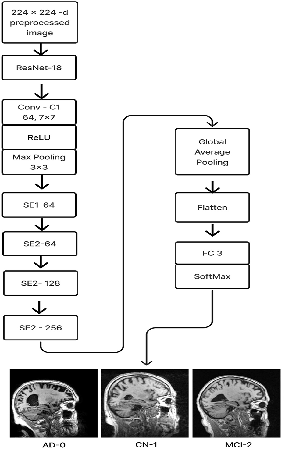
Figure 8. Proposed model 2: ResNet-18 pre-trained model with SE block.

The ResNet-18 pretraining model initializes the weights (ImageNet) of 17 convolutional layers, with the exception of SE-Block (Gao et al., 2021), during the training phase. Once the learned weights were loaded, the entire model was retrained using the current ADNI dataset. This can increase training speed and accuracy and enhance the model's ability to detect illness stages from the existing MRI image collection. For feature learning to be steady and successful, this is essential. The Squeeze and Excitation components make up the ResNet-18 pre-trained model with SE. Every SE block adaptively re-calibrates channel-wise feature responses by simulating channel interdependencies and embedding the knowledge globally. ResNet-18, the pre-training model, was used as the first layer, and the last fully connected layer of the ResNet-18 model was replaced by four SE blocks integrated as the next four layers. After that, the features were flattened and averaged. Ultimately, a fully connected layer made up of three neurons with a softmax activation function is link