1 Introduction

High-fidelity reconstruction of electroencephalography (EEG) data is of key relevance to many deep learning (DL) tasks for EEG analysis, such as anomaly detection, automatic labeling, classification, and brain-computer interface control (Kodama et al., 2023; Beraldo et al., 2022). The most significant open challenges for the DL models are the complex dynamics of the EEG signals and the large inter-subject variability. So far, these two aspects have prevented DL to offer a gold-standard for high-accurate reconstruction of multi-channel EEG data (Lotte et al., 2018). A critical issue for DL methods is the dependency on the training set, as Gyori et al. (2022) recently pointed out in the domain of magnetic resonance imaging data: a training dataset of poor quality, as well as a training set distributed in a non-representative way might induce biases in the trained model and, consequently, lead to poor results in the task the model is expected to perform e.g., classification or anomaly detection. At the same time, in the neuroscience domain, it is very common to meet this situation (Pion-Tonachini et al., 2019), as the complex dynamics of any biological signal and the large inter-individual variability make it difficult to obtain a clean, large, and representative training set.

Nonetheless, in this paper, we present a novel deep learning model, called hvEEGNet, designed as a hierarchical variational autoencoder (VAE), where the encoder and the decoder modules have been inspired by the popular EEGNet architecture (Lawhern et al., 2016). The proposed model was trained by using a novel loss function based on dynamic time warping (DTW), never used before for EEG data, but very well-suited for time-series (Bankó and Abonyi, 2012). We show that the combination of this specific architecture and the training strategy brings to high-fidelity reconstruction of multi-channel EEG signals. Interestingly, this is also consistent across different subjects. To test our model, we use a benchmark dataset called dataset 2a to have a fair comparison with previous works. Then, we deepen the investigation of the model's training over this particular dataset, and we empirically observe that there is a relationship between the training time (i.e., the number of epochs needed to train the model for each subject) and the particular distribution of the EEG values in each subject. We show that 80 epochs are enough to obtain almost perfect reconstruction for all subjects in the dataset, but for some of them 20 epochs are sufficient. Thus, with this work, we shed light on the importance of conducting a systematic analysis of the input EEG data and its variability across different subjects to ensure proper DL models training, a step never reported by previous works (as far as the authors know).

In this paper, we provide the following novel contributions:

1. we show that the choice of DTW as the loss function, in place of the more standard mean square error (MSE), has a key role in the accurate EEG reconstruction;

2. a simple VAE model cannot properly recover multi-channel EEG data, while a hierarchical architecture (i.e., hvEEGNet) provides high-fidelity reconstruction;

3. hvEEGNet is trained very fastly, in a few tens of epochs, despite the small size of the training dataset;

4. finally, using the trained model (in a within-subject modality), we discovered some significant instrumental anomalies in the benchmark dataset (never pointed out before).

2 State of the art

Reconstructing a multi-channel EEG dataset with high-fidelity is a challenging task, given the typical very low signal-to-noise ratio characterizing EEG signals (Cisotto, 2021), the fast dynamics of each signal and its relationship with signals acquired from different locations of the scalp, and the large inter-subject variability (both between healthy and patients, but also across different individuals sharing the same condition). So far, even with the development of DL techniques, there is no gold-standard model available to obtain a general-purpose high-fidelity EEG reconstruction. From the most recent literature, two main trends can be highlighted: on one side, some recent works proposed DL models to reconstruct multi-channel EEG, but they can only achieve poor reconstruction quality. For example, Bethge et al. (2022) proposed EEG2VEC, i.e., a VAE architecture to encode emotions-related EEG signals in the VAE latent space. The authors succeeded in reconstructing the low-frequency components of the original EEG signals but the higher frequency ones were not properly recovered. Moreover, the output signals appeared to be largely attenuated (amplitudes often halved w.r.t. the original ones). According to the authors' explanation, this was due to the particular design of the decoder which might have introduced aliasing and artifacts. In one of the our previous work (Zancanaro et al., 2023a), we also found similar results. There, we proposed vEEGNet-ver1, a new VAE architecture designed to extract latent representations of multi-channel EEG both to classify EEG signals [via feed-forward neural network (FFNN)] and to reconstruct them. We achieved state-of-the-art classification performance, but only poor reconstruction: specifically, we were able to retrieve only a slow frequency component [related to the initiation of the movement (Bressan et al., 2021; Ofner et al., 2019)] but we failed to recover higher frequencies information. On the other side, other works (Al-Marridi et al., 2018; Dasan and Gnanaraj, 2022; Khan et al., 2023; Liu et al., 2020) were able to reconstruct EEG signals with high accuracy but from a single-channel acquisition setup. They mostly dealt with single-channel reconstruction with the perspective of compression in wireless portable devices. In Al-Marridi et al. (2018), the authors implemented a convolutional autoencoder to compress EEG signals, showing good abilities to reconstruct single channel EEG signals with a relatively high compression ratio (up to 98% with distortion of 1.33%). Dasan and Gnanaraj (2022) proposed a multi-branch denoising autoencoder to compress EEG signals coming from one only sensor, together with the Electrocardiogram (ECG) and electromyographic (EMG) signals coming from other two sensors with the purpose to ensure continual learning (continuous fine-tuning) and real-time health monitoring. Each signal modality (EEG, Electrocardiogram (ECG), electromyographic (EMG)) was independently pre-processed, and then the autoencoder provided a multi-modal latent representation. The results showed a good trade-off between compression ratio and reconstruction quality over three public datasets. This work represents an interesting approach, but it assumes to have complementary information about the subjects (their muscular and heart activity). Also, this approach can be adopted in those applications where movement is involved, but it might be more difficult to apply with pure cognitive tasks (e.g., imagination of the movement or sleeping). Lastly, it might also be expected that the use of portable devices bring lower EEG signal quality (typically capturing lower frequencies), thus making the final recovery easier. Finally, Khan et al. (2023) used a shallow autoencoder with a low dimensional latent space (8–64) to classify single-channel EEG signals of a public dataset into epileptic vs. healthy classes, achieving 97% accuracy, sensitivity and specificity over 96%. They also achieved very good reconstruction, as shown in two representative signals. Unfortunately, the authors did not report the power spectrum of the original EEG signals, thus making it difficult to fully ensure a reproducibility of these good performance on other, more complex (i.e., with larger bandwidth), EEG data. In Liu et al. (2020), an autoencoder was trained within a larger deep learning architecture with the goal of compressing and reconstructing the EEG data. Particularly, its input is given by the output of a convolutional neural networks (CNN), used as feature extractor. The CNN and the autoencoder were trained together. Then, the optimized features were fed to a FFNN that operated a classification (with separate training). They tested their model on the very popular DEAP (Koelstra et al., 2012) and SEED (Zheng and Lu, 2015) public emotions-related EEG datasets, reaching satisfactory results (accuracy around 90% in both arousal and valence categories for DEAP, and over 96% for the three classes of SEED). However, the authors did not provide results about the quality of the reconstruction of the autoencoder. It can be said that most literature is focused on using DL techniques to solve application-tailored classification problems. However, a systematic investigation to extract more general conclusions on the reconstruction effectiveness of those models is still lacking.

Similar considerations hold true about the application of DL for the detection of anomalies in EEG, a natural related application of high-fidelity reconstruction. The vast majority of the studies at the state-of-the-art have targeted the automatic identification of pathological events (e.g., seizures) w.r.t. certified, artifact-free, and healthy EEG signals. In this task, autoencoders have been largely and successfully employed, as they offer the inherent possibility to be used as anomaly detectors (Pang et al., 2021), provided that they can learn from good quality training data. As an example, Emami et al. (2019) showed that a model based on an autoencoder and a threshold labeling system can detect epileptic seizures with 100% accuracy in about 92% cases (22 subjects over 24 of a private dataset). Ortiz et al. (2020) reached similar outstanding results (accuracy of 96%, sensitivity of 86%, specificity of 100%, area under the curve (AUC) of 92%) using a cascaded system with an autoencoder trained to reconstruct the time-series of some handcrafted features to enhance the spatial differences in the brain activity of patients suffering from dyslexia and healthy controls [a support vector machine (SVM) later classifies the two classes].

Nevertheless, there is no well-established definition of normality for EEG signals, as much as it is fairly difficult to have a certified, large, and artifact-free dataset (even in the case of healthy subjects) (Gabardi et al., 2023). Therefore, it would be more realistic to train an autoencoder model on a mixture of clean and noisy data, in line with some other literature (not necessarily addressing biological data). For instance, in Zhou and Paffenroth (2017), the authors proposed a robust autoencoder, i.e., a combination of a robust PCA (RPCA) and an autoencoder, where the autoencoder was used for data projection in the (reduced) principal components space (in place of the usual linear projection). Unfortunately, there is a limited literature on this kind of autoencoders, as confirmed by a recent survey (Al-amri et al., 2021). In Xing et al. (2020), the authors proposed a combination of an evolving spiking neural network and a Boltzmann machine to identify anomalies in a multimedia data stream. The proposed training algorithm was able to localize and ignore any random noise that could corrupt the training data. In Dong and Japkowicz (2018), a model composed by an ensemble of autoencoders was employed to identify anomalies in data streams. The authors claimed that the training algorithm made the presence of noisy samples in the training data not statistically significant, thus ensuring model's robustness to noise. In Qiu et al. (2019), an architecture made by the sequence of a CNN, an long-short term memory (LSTM), a FFNN, and a softmax layer was proposed to identify anomalies. Interestingly, a VAE was preliminarily used to over-sample the dataset, before training the classifier (i.e., the FFNN with the softmax layer). The model was tested on the AIOps-KPI public dataset (Li et al., 2022), achieving an accuracy of 77% (KP1), 75% (KP2), 83% (KP3), and 75% (KP4). Nevertheless, to the best of our knowledge, this kind of approaches has never been applied to EEG data, yet.

Thus, some fundamental open challenges emerge from the state of the art (SOTA) review to be solved, including (1) the high reconstruction errors or the generation of traces that are not faithful to the original signals, (2) the lack of focus on the reconstruction task (in favor of classification or anomaly detection) even if the architecture has this possibility, and (3) no rigorous investigation on the impact of the input quality and distribution on the training of DL models. Thus, in this paper we shed light on these important challenges in relation to high-fidelity reconstruction of multi-channel EEG data.

3 Materials and methods

In this section, we present the basic modules as well as the overall architecture of our proposed model, hvEEGNet. Also, to support our design choices, we introduce another model, namely vEEGNet-ver3, which shares the same new loss function with hvEEGNet, but a different (simpler, i.e., not hierarchical) architecture. Furthermore, we describe the metrics and the methodologies we employed to evaluate our models.

3.1 Variational autoencoder

The common overall architecture of our both models is the VAE.

Unlike traditional autoencoders, i.e., producing a deterministic encoding for each input, VAE is able to learn a probabilistic mapping between the input data and a latent space, which is additionally learned as a structured latent representation (Kingma and Welling, 2013, 2019). Given the observed data x and assuming z to be the latent variables, with a proper training, a VAE learns the variational distribution qϕ(z|x) as well as the generative distribution pθ(x|z), using a pair of (deep) neural networks (acting as the encoder and the decoder), parameterized by ϕ and θ, respectively (Blei et al., 2017). The training loss function, denoted as LVAE, accounts for the sum of two different contributions: the Kullback-Leibler divergence between the variational distribution qϕ(z|x) and the posterior distribution pθ(x|z), denoted as LKL, and the reconstruction error, denoted as LR, which forces the decoded samples to approximate the initial inputs. Thus, the loss function adopted for the VAE is

LVAE=LKL+LR=-KL[qϕ(z|x)||p(z)]+?q(logpθ(x|z))    (1)

Assuming normal distribution as a prior for the sample distribution in the latent space, it is possible to rewrite Equation 1 as follows

LVAE=−12∑i=1d(σi2+μi2-1-log(σi2))+?q(logpθ(x|z))    (2)

where μi and σi2 are the predicted mean and variance values of the corresponding i-th latent component of z.

In this work, we adopted this basic architecture to propose vEEGNet version 3 (vEEGNet-ver3). The details characterizing this specific model are reported in Section 3.3.

3.2 Hierarchical VAE

A hierarchical VAE (Vahdat and Kautz, 2021) is the evolution of a standard VAE enriched by a hierarchical latent space, i.e., multiple layers implementing a latent space each. In fact, standard VAEs suffer from the lack of accuracy in details reconstruction, given by the trade-off between the reconstruction loss and the Kullback-Leibler divergence contributions, thus generating the tendency to generate slightly approximated data (e.g., blurred images), only. Hierarchical VAEs attempt to solve this problem by using multiple latent spaces, where each of them is trained to encode different levels of detail in the input data. Assuming a model with L latent spaces, its loss function can be written as

where

LKL=-KL[qϕ(z1|x)||p(z1)]-∑l=2LKL[qϕ(zl|x,z<l)||p(zl|z<l)],    (4)

with qϕ(zl|,z<l)=∏i=1l-1qϕ(zl|x,z<i) as the approximate posterior up to the (l−1) level and the conditional in each prior p(zl|z<l) and approximate posterior qϕ(zl|x, z < i) is represented as a factorial normal distribution. The notation is taken from the original paper (Vahdat and Kautz, 2021). Particularly, the symbol z<i means that the random variable is conditioned by the output of all latent spaces from 1 to i.

In this work, we adopted this basic architecture to propose hierarchical vEEGNet (hvEEGNet). The details characterizing this specific model are reported in Section 3.5.

3.3 vEEGNet-ver3

Figure 1 represents the schematic architecture of this simple VAE model. As any conventional VAE, it consists of an encoder, a latent space, and a decoder.

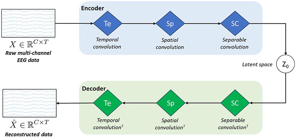
Figure 1. Schematic architecture of our model called vEEGNet-ver3. The encoder block is formed by three blue diamonds representing three different processing layers: i.e., Te stands for temporal convolution, Sp stands for spatial convolution, and SC stands for separable convolution. The decoder block includes three green diamonds representing the same operations, in the reverse order and using the transpose convolution (T). z0 represents the latent space.

However, inspired by the work of Lawhern et al. (2016), we designed the encoder as the popular EEGNet architecture, i.e., with the three processing blocks: in the first block, a horizontal convolution (that imitates the conventional temporal filtering) is followed by a batch normalization. In the second block, a vertical convolution, acting as a spatial filter, is applied. This operation is then followed by an activation and an average pooling step. The third, and last, block performs a separable convolution with a horizontal kernel, followed by an activation and an average pooling step. We always used, as in Lawhern et al. (2016), the exponential linear unit (ELU) activation function. At the output of the third block, the obtained D × C × T tensor is further transformed by means of a sampling layer which applies a convolution with a 1 × 1 kernel, thus doubling its depth size, resulting in a 2D × C × T tensor. Finally, the latter is projected onto the latent space (i.e., of dimension N = D·C·T). In line with other previous works (Zancanaro et al., 2023a; Kingma and Welling, 2013), the first N elements of the depth map were intended as the marginal means (μ) and the second N elements as the marginal log-variances (σ) of the Gaussian distribution represented in the latent space. Then, to reconstruct the EEG data, the latent space z0 is sampled using the reparameterization trick, as follows:

where N(0, 1) is standard multivariate Gaussian noise (with dimension N = D·C·T).

Finally, in the projection onto the latent space, we apply a 1 × 1 convolution to the output of the encoder, thus obtaining a depth map whose first half is taken as the mean and the second half as the log-variance of the distribution of the latent space.

To note, this architecture is very similar to other previous architectures proposed by the authors in Zancanaro et al. (2023a) and in Zancanaro et al. (2023b). However, it introduces a very significant novelty that leads this new model to perform much better than the older ones. The reconstruction error LR of the VAE loss function expressed by Equation 1 was here quantified by the DTW similarity score (Sakoe and Chiba, 1978), i.e., replacing the more standard MSE. DTW leads to a more suitable measure of the similarity between two time-series (Bankó and Abonyi, 2012), thus allowing the model better learn to reconstruct EEG data. In fact, DTW is known to be more robust to non-linear transformations of time-series (Huang and Jansen, 1985), thus capturing the similarity between two time-series even in presence of time shrinkage or dilatation, i.e., warpings. This cannot be achieved by MSE, which is highly sensitive to noise, i.e., the error computed by MSE rapidly increases when small modifications are applied to time-series.

3.4 DTW and normalized DTW

In brief, given two time-series a(i) and b(j), where i, j = 1, 2, ..., T (i.e., for simplicity, we consider two series with the same length), DTW is a time-series alignment algorithm that extensively searches for the best match between them, by following a five-step procedure:

1. The cost matrix W is initialized, with each row i associated with the corresponding amplitude value of the first time-series a(T − i + 1), while each column j associated with the corresponding amplitude value of the second time-series b(j).

2. Starting from position W(0, 0), the value of each matrix element is computed as W(i, j) = |a(i) − b(j)| + min[W(i − 1, j − 1), W(i, j − 1), W(i − 1, j)], if i, j > 0, otherwise W(i, j) = |a(i) − b(j)|.

3. The optimal warping path is identified as the minimum cost path in W, starting from the element W(1, T), i.e., the upper right corner, ending to the element W(T, 1).

4. the array d is formed by taking the values of W included in the optimal warping path. Note that d might have a different (i.e., typically longer) length compared to the two original time-series, as a single element of one series could be associated with multiple elements of the other.

5. Finally, the normalized DTW score is computed as

where K is the length of the array d. To note, normalization was not applied during the models' training (to keep this contribution in the range of the other loss function contributions). Whereas, during the performance evaluation, we used the normalized score. Nevertheless, this difference did not induce criticisms, as all segments share the same length.

3.5 hvEEGNet

As we observed sub-optimal reconstruction results with vEEGNet-ver3 and in line with other literature on computer vision (Vahdat and Kautz, 2021), we developed a new architecture, called hvEEGNet, to overcome the issues of vEEGNet-ver3. The most relevant change in hvEEGNet w.r.t. vEEGNet-ver3 is its hierarchical architecture with three different latent spaces, namely z1, z2, and z3, with z1 being the deepest one. Each of them is located at the output of each main block of the encoder, i.e., after the temporal convolution (Te) block (z3), after the spatial convolution (Sp) block (z2), and after the separable convolution (SC) block (z1). The input to the decoder's Sp block is now given by the linear combination (i.e., the sum) of the SC block's output and the sampled data from z2. Similarly, the input to the decoder's Te block is obtained by the sum of the Sp block's output and the sampled data from z3. Incidentally, but significantly, it is worth noting that we kept here using the DTW algorithm to compute the reconstruction loss LR (with reference to Equation 5). The main structure of the model is depicted in Figure 2.

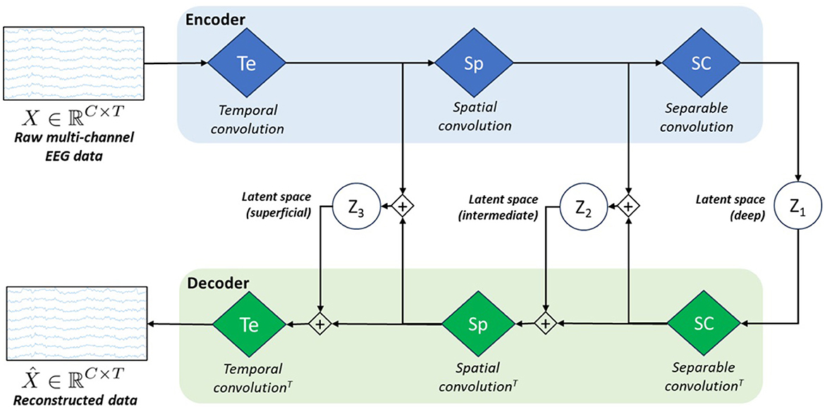
Figure 2. Schematic architecture of our model called hvEEGNet. The encoder block is formed by the same three processing layers (i.e., blue diamonds) as in vEEGNet-ver3 (Figure 1). The decoder block includes three green diamonds representing the same operations, in the reverse order and using the transpose convolution (T). z1, z2, and z3 represent the latent spaces obtained at the three different processing levels.

Tables 1 and 2 report the details of both vEEGNet-ver3 and hvEEGNet architectures.

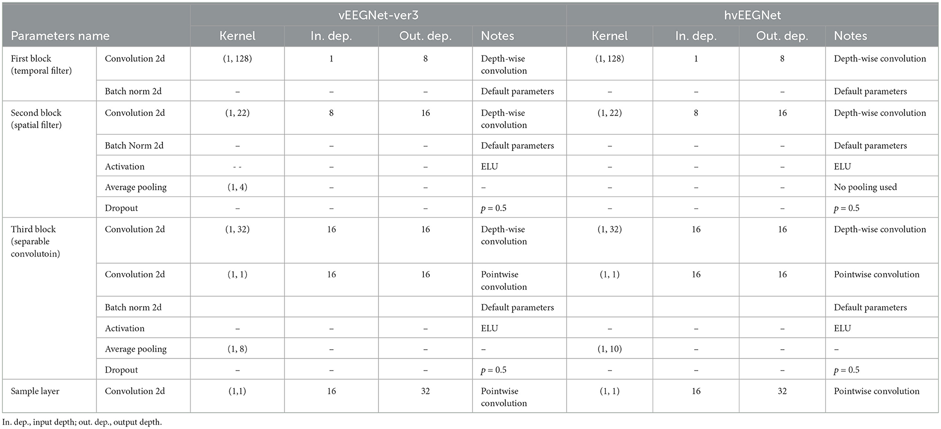
Table 1. Parameters' values of the vEEGNet-ver3's and hvEEGNet's encoder, respectively.

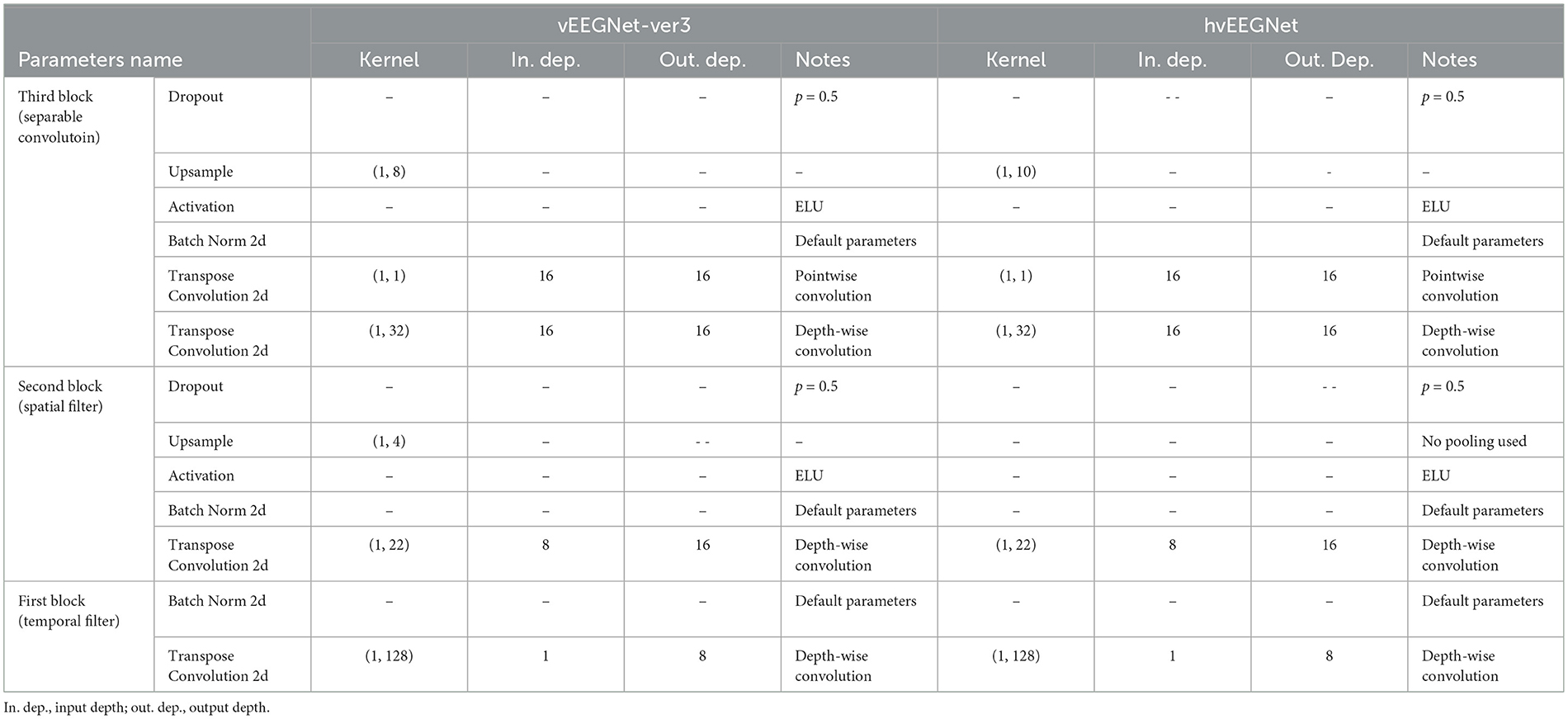
Table 2. Parameters' values of the vEEGNet-ver3's and hvEEGNet's decoder, respectively.

3.6 Outlier identification

As our architectures implement completely self-supervised models, we have the opportunity to use them as anomaly detectors. In line with the vast majority of related work (as introduced in Section 2), in the present study, we define as an outlier any sample (i.e., EEG segment) that is very poorly reconstructed. This, in turn, is verified by large values of the DTW similarity score between the reconstructed EEG sample and the original one. To identify such samples, we decided to use the k-nearest neighbors (kNN) algorithm (Cover and Hart, 1967). kNN is an unsupervised machine learning (ML) algorithm that computes the distance between every sample and its k-th nearest neighbor (with k properly chosen). All samples in the dataset are sorted w.r.t. increasing values of such distance. Those points whose distance (from their k-th nearest neighbor) exceeds a user-defined threshold are labeled as outliers.

In the second part of this study, we used hvEEGNet model to identify the outliers. Before applying kNN, we performed two pre-processing steps: we computed the DTW similarity score for the EEG segment (i.e., channel- and repetition-wise). To note, by definition (see Equation 5), the score is normalized by the number of time points in the series (even though all time-series have fixed length in this work). For each training run, we built the following matrix E:

E(t)=[e11(t)e12(t)⋯e1C(t)e21(t)⋱⋯⋮⋮⋮⋱⋮eR1(t)⋯⋯eRC(t)]    (5)

with t = 1, 2, ..., T, given T the number of training runs, r = 1, 2, ..., R, with R the number of segments (i.e., task repetitions), and c = 1, 2, ..., C, with C the number of EEG channels. Then, erc(t) represents the normalized DTW value obtained from the reconstruction of the r-th segment at the c-th channel after training the hvEEGNet model in the t-th training run. Finally, the matrices E(t), with t = 1, 2, ..., T are averaged to obtain E¯, and then kNN is applied. Also note that kNN took every sample of the dataset as defined by a C-dimensional EEG segment (i.e., one row in matrix E¯). This allowed us to identify two types of outliers: (1) repetitions where all (or, the majority of the) channels were affected by some mild to severe problem, or (2) repetitions where only one (or, a few) channel was highly anomalous. Both are very common situations that might occur during neuroscience experiments (Teplan et al., 2002).

3.7 Implementation

We employed PyTorch to implement and to design and train our models.

To implement the newly proposed loss function, i.e., including the DTW computation, we exploited the soft-DTW loss function CUDA time-efficient implementation (available at: https://github.com/Maghoumi/pytorch-softdtw-cuda) (Maghoumi, 2020; Maghoumi et al., 2021). In fact, the original DTW algorithm is quite time-consuming and employs a minimum function that is non-differentiable. Then, in Cuturi and Blondel (2017), a modification of the original algorithm was proposed to specifically be used in DL models, i.e., to be differentiable, thus suitable as a loss function. Then, CUDA was employed to make it time-efficient, too. Also, it is worth noting that DTW works with 1D time-series. However, our models aimed to reconstruct multi-channel EEG time-series. Then, during training, we computed the channel-wise DTW similarity score between the original and the reconstructed EEG segment. Then, in the loss function, we added the contribution coming from the sum of all channel-wise DTW scores.

The models were trained using the free cloud service offered by Google Colab, based on Nvidia Tesla T4 GPU. The hyperparameters were set as follows: batch size to 30, learning rate to 0.01, the number of epochs to 80, an exponential learning rate scheduler with γ set to 0.999. Twenty training runs for each subject, were performed, in order to better evaluate the stability of the models training and the error trend along the epochs. The total number of parameters of the vEEGNet-ver3 is 4, 992 and the state dictionary (i.e., including all parameter weights) is 40kB-weight. The total number of parameters of the hvEEGNet model is 8,224, with 5, 456 of them to define the encoder, and the remaining 2, 768 for the decoder. Note that the higher number of parameters in the decoder is due to the sampling layers that operate on the three different latent spaces. The state dictionary of the parameter weights is about 56kB.

Finally, for the kNN algorithm for outliers detection (see Section 3.6), we employed the well-known knee method in the implementation given by the kneed python package (Satopaa et al., 2011) to find the threshold distance to actually mark some samples as outliers.

To foster an open science approach to scientific research, we made our code available on GitHub (at: https://github.com/jesus-333/Variational-Autoencoder-for-EEG-analysis).

3.8 Performance evaluation

In this work, we evaluated our models in a within-subject scenario (Zancanaro et al., 2021), only. Cross-subject evaluations, even though possible, are left for future developments as they deserve an entire new campaign of experiments and analyses.

The evaluation was carried on based on two different approaches: first, visual inspection of the reconstructed data in both the time and frequency domains (with the most convenient frequency range selected figure by figure); second, the quantification of the average reconstruction quality using the normalized DTW similarity score, as defined in Equation 5.

For visual inspection, we compared in a single plot the time domain representations of the original EEG segment and its corresponding reconstructed one. Also, we computed the Welch's spectrogram (Welch, 1967) (in the implementation provided by the Python Scipy package, available at: https://docs.scipy.org/doc/scipy/reference/generated/scipy.signal.welch.html) with the following parameters: Hann's window of 500 time points with 250 time points overlap between consecutive segments.

Then, to train and test our models (both vEEGNet-ver3 and hvEEGNet), we inherited the same split proposed by Blankertz et al. (2007): for every subject, 50% data were used for the training and the remaining 50% (i.e., a later experimental session) for the test. Furthermore, we applied cross-validation using 90% of the training data for the actual models' training and 10% for the validation. With the aim of investigating the training behavior of our models w.r.t. the particular input dataset, we repeated 20 training runs for each subject (i.e., each run started from a different random seed, thus ensuring a different training/validation split in the overall training set). This allowed us to provide a more robust evaluation of the training curve along the training epochs. We reported the models' performance in terms of descriptive statistics (mean and standard deviation across multiple training runs) of the reconstruction error along the training epochs (i.e., in other words, the training time). To note, in some rare cases where the loss function's gradient could not be minimized, we excluded those training runs from our final evaluation and training visualization.

Finally, the reconstruction ability of our models, after proper training (i.e., 80 epochs), was evaluated on the test set, too, by means of the same normalized DTW similarity score.

4 Results and discussion 4.1 Dataset

Dataset 2a of BCI Competition IV (Blankertz et al., 2007) was downloaded using the MOABB tool (Jayaram and Barachant, 2018) and it is composed by the 22-channel EEG recordings of nine subjects while they repeatedly performed four different motor imagery (MI) tasks: imagination of the movement of the right hand, left hand, feet or tongue. Each repetition consists of about 2 s fixation cross task, where a white cross appeared on a black screen and the subject needed to fix it and relax (as much as possible). Then, a 1.25 s cue allowed the subject to start imagining the required movement. The cue was displayed as an arrow pointing either left, right, up, or down, to indicate the corresponding task to perform, i.e., either left hand, right hand, tongue, or feet MI. MI was maintained until the fixation cross disappeared from the screen (for 3 s). A random inter-trial interval of a few seconds was applied (to avoid subjects habituation and expectation). Then, several repetitions of each type of MI were required to be performed. The order to repeat the different MI tasks was randomized to avoid habituation. The timeline of the experimental paradigm can be found in the original work by Blankertz et al. (2007).

A total number of 576 trials (or, repetitions) was collected from each individual subject. The EEG data were recorded with a sampling frequency of 250 Hz and the authors filtered the data with a 0.5 − 100Hz band-pass filter and a notch filter at 50 Hz (accordingly to the experimental records associated with the public dataset). We kept these settings as they were, to be in line with the literature (Lawhern et al., 2016) and to be consistent with our previous studies (Zancanaro et al., 2021, 2023a,b).

As explained in Section 3.8, we adopted the pre-defined 50/50 training/test split on the dataset and thus, for each subject, we obtained 260 EEG segments for the training set, 28 for the validation set, and 288 for the test set. To note, the dataset was perfectly balanced in terms of stratification of the different subjects in all splits.

We performed segmentation and, for each MI repetition, we extracted a 4s (22-channel) EEG segment. The piece of EEG was selected in the most active MI part of the repetition, i.e., from 2 to 6s, in order to isolate the most apparent brain behavior related to the MI process. Figure 3 shows an example of two raw EEG signals, represented both in the time domain and in the frequency domain (with the frequency range limited to 50 Hz for visualization purposes). To note, to improve visualization in the time domain, the signals are shown in the limited time range from 2 to 4s. However, in the frequency domain, the entire 4 s segment was used to compute the power spectrum (via Welch method, as described in Section 3.8). Then, a total of 1, 000 time points are included in each EEG segment.

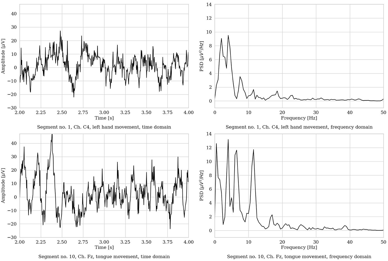
Figure 3. Two representative EEG segments from the Dataset 2a from S3 (time range limited from 2 to 4 s, frequency range limited to 50 Hz). (Left) Time domain representation. (Right) Frequency domain representation.

4.2 Reconstruction performance

In this section we show the performance of vEEGNet-ver3 and hvEEGNet, and we discuss to what extent the new loss function (with the DTW contribution) and the hierarchical architecture influenced the reconstruction performance.

First, we visually inspect the output from our two models. Figure 4 shows a representative example of one EEG segment as reconstructed by vEEGNet-ver3 and hvEEGNet, respectively, in both the time and the frequency domain (with the frequency range extended to 80 Hz for visualization purposes).

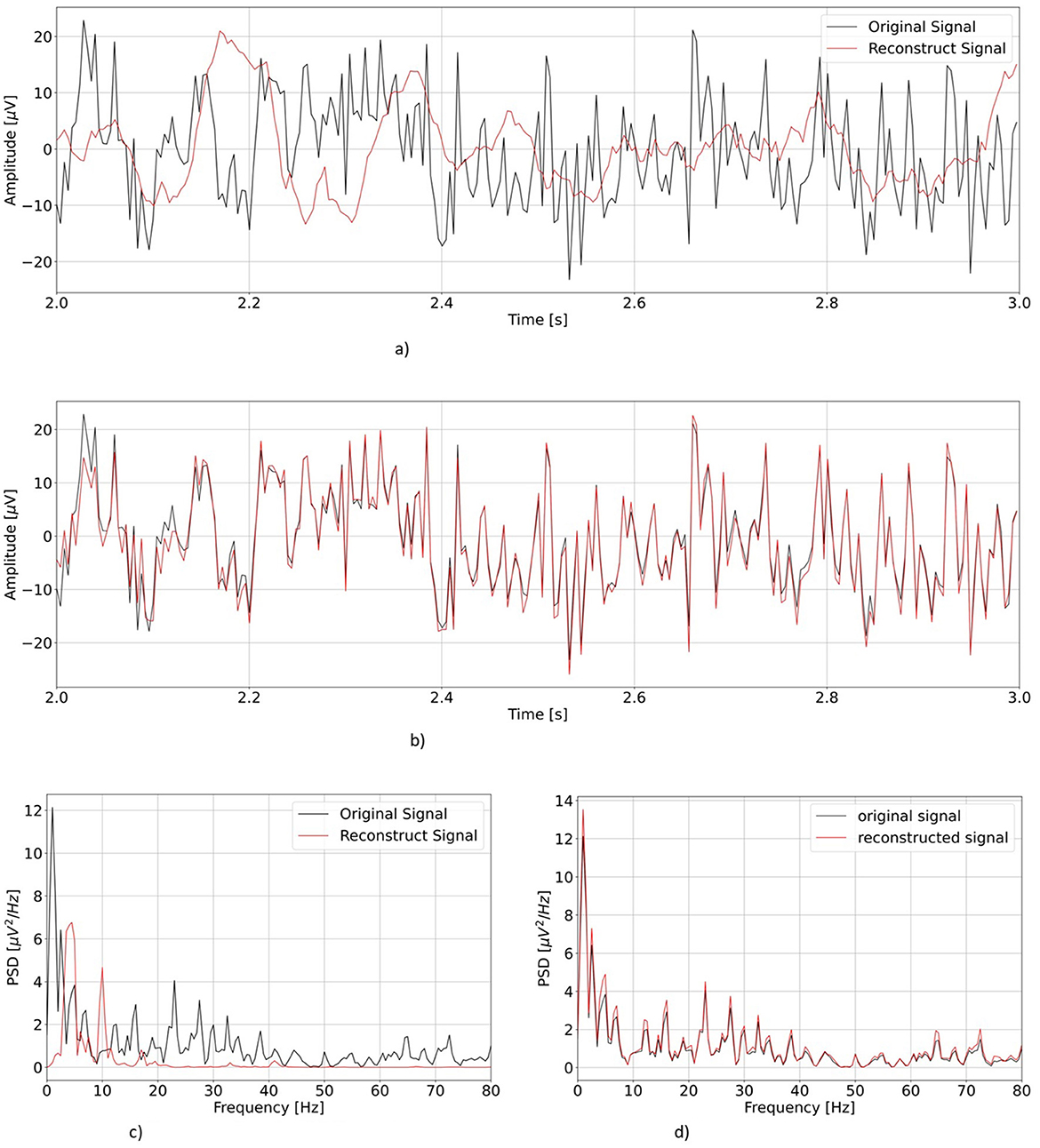
Figure 4. Comparison of the re