1 Introduction

Epilepsy is a chronic neurological disorder affecting over 50 million people worldwide, according to the World Health Organization. It can impact individuals of all ages and is characterized by recurrent seizures, which result from sudden, abnormal discharges of neurons in the brain (Pelkonen et al., 2020). These seizures can vary widely in severity and presentation, ranging from brief lapses in awareness to full-body convulsions. The underlying causes of epilepsy are diverse, including genetic, infectious, structural, immune, metabolic, and sometimes unknown factors (Scheffer et al., 2017). The primary treatments for epilepsy include medication and surgery, but these interventions are not always effective (Perucca, 2021). Approximately 30% of patients continue to experience recurrent seizures despite treatment (Liu et al., 2021). These seizures can lead to a range of symptoms, including loss of consciousness, muscle twitching, and difficulty breathing (World Health Organization, 2024). In severe cases, seizures can result in falls, injury, and even drowning, posing significant risks to life. Additionally, the social implications of epilepsy, such as the potential for discrimination and the stigma associated with the condition, can exacerbate psychological distress. Studies have shown that individuals with epilepsy, especially children and adolescents, are more likely to suffer from anxiety and depression due to the chronic and unpredictable nature of their condition (Puka et al., 2017). EEG, which records the brain’s electrical activity, is a crucial tool in diagnosing and managing epilepsy. However, analyzing EEG data is time-consuming and requires the expert of trained neurologists. The accuracy of diagnosis heavily depends on the neurologist’s experience and skill. This traditional approach has its limitations: particularly given the complexity and volume of EEG data that must be reviewed (Chandani and Kumar, 2018). In recent years, the development of deep learning techniques has offered new possibilities for improving epilepsy detection and prediction. These advanced algorithms can process and analyze large volumes of EEG data more efficiently than traditional methods, assisting neurologists in diagnosing epilepsy and predicting seizures more accurately. By providing timely warnings, these technologies can help patients take preventive measures, reducing the physical and psychological impact of seizures. This paper provides a comprehensive review of the current research on epileptic EEG signal detection and prediction using deep learning methods. EEG has the advantages of simplicity, safety, high temporal resolution, and high utilization, making it a key tool in diagnosing epilepsy (Wei et al., 2021; Ein Shoka et al., 2023). Given this prevalence, this paper concentrates on reviewing literature specifically related to EEG signals in the context of epilepsy. We will explore four key areas: the nature of epileptic EEG data, preprocessing techniques, feature extraction methods, and deep learning-based detection and prediction algorithms. This review also addresses gaps in existing literature, including issues related to data partitioning, model evaluation methods, and prediction timeframes, offering a more detailed perspective on the state of the field.

2 Epileptic EEG signals 2.1 Partitioning of epileptic EEG signal states

EEG signals of an epileptic patient can be categorized into four states: Post-ictal state, Inter-ictal state: Pre-ictal state and Ictal state. The pre-ictal state is the state minutes before the actual occurrence of the seizure. The ictal state is the state actual occurrence of the seizure. The post-ictal state is the state after the seizure has passed. The inter-ictal state is the state between post-ictal state and preictal state. Signals during ictal and inter-ictal periods are often used as data for detecting the occurrence of epilepsy. Signals during pre-ictal and inter-ictal periods are often used as data to predict whether epilepsy will occur or not (Aslam et al., 2022). Figure 1 illustrates the four states of epileptic EEG signals.

Figure 1. Four states of epileptic EEG signals.

2.2 Data presentation

The 10–20 International Standard Electrode Placement System, established by the International Federation of Clinical Neurophysiology, is widely recognized as the standard method for electrode placement in EEG data acquisition (Maillard and Ramantani, 2017). This system is employed by most publicly available epileptic datasets, ensuring consistency and reliability in data collection. In this section, we will discuss commonly used datasets in epilepsy research. Most of these datasets are freely accessible, with the exception of the Bonn dataset, which requires a purchase. These datasets typically organize epileptic EEG data on a patient-by-patient basis, with each patient’s data stored in separate folders. This organization leads to two primary methods of data segmentation for epilepsy detection and prediction: patient-independent and non-patient-independent methods.

Patient-independent methods refer to data from a particular patient as training, validation, and testing data for the model. This data partitioning approach can be further divided into two types: segment-based approach and event-based approach. Segment-based approach means that the data of a particular patient is divided into training, validation, and testing sets. The event-based approach means: dividing the data of a patient into k groups according to the number of seizures, using the k-1 group of data as the training and validation set, and the kth group of data as the test set. This approach generally yields more accurate evaluation results compared to non-patient-independent methods. However, it requires a substantial amount of patient-specific data, which must be recorded over different seizure periods to effectively train the model for detecting or predicting seizures in that particular patient. Figure 2A shows the segment-based data partitioning method and Figure 2B shows the event-based data partitioning method.

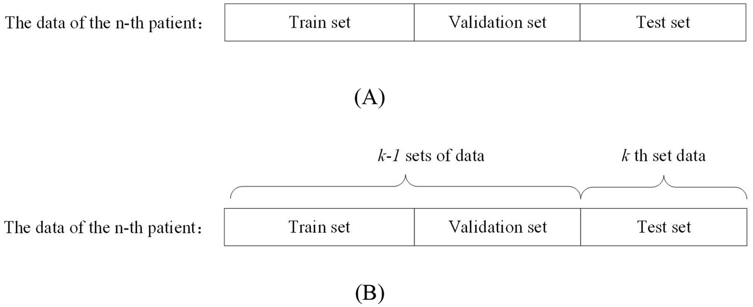
Figure 2. Schematic diagram of patient-independent data segmentation.

On the other hand, non-patient-independent methods refer to the use of all patients’ data as training, validation, and testing data for the model. This data partitioning can be further divided into two types: the all-patient approach and the cross-patient approach. The difference is as follows: the all-patient approach divides data from all patients into training, validation, and testing sets. The cross-patient approach refers to dividing the data of n-1 patients as the training set and validation set, and the remaining patient data as the test set. Figure 3A shows the all-patient data division method and Figure 3B shows the cross-patient data division method.

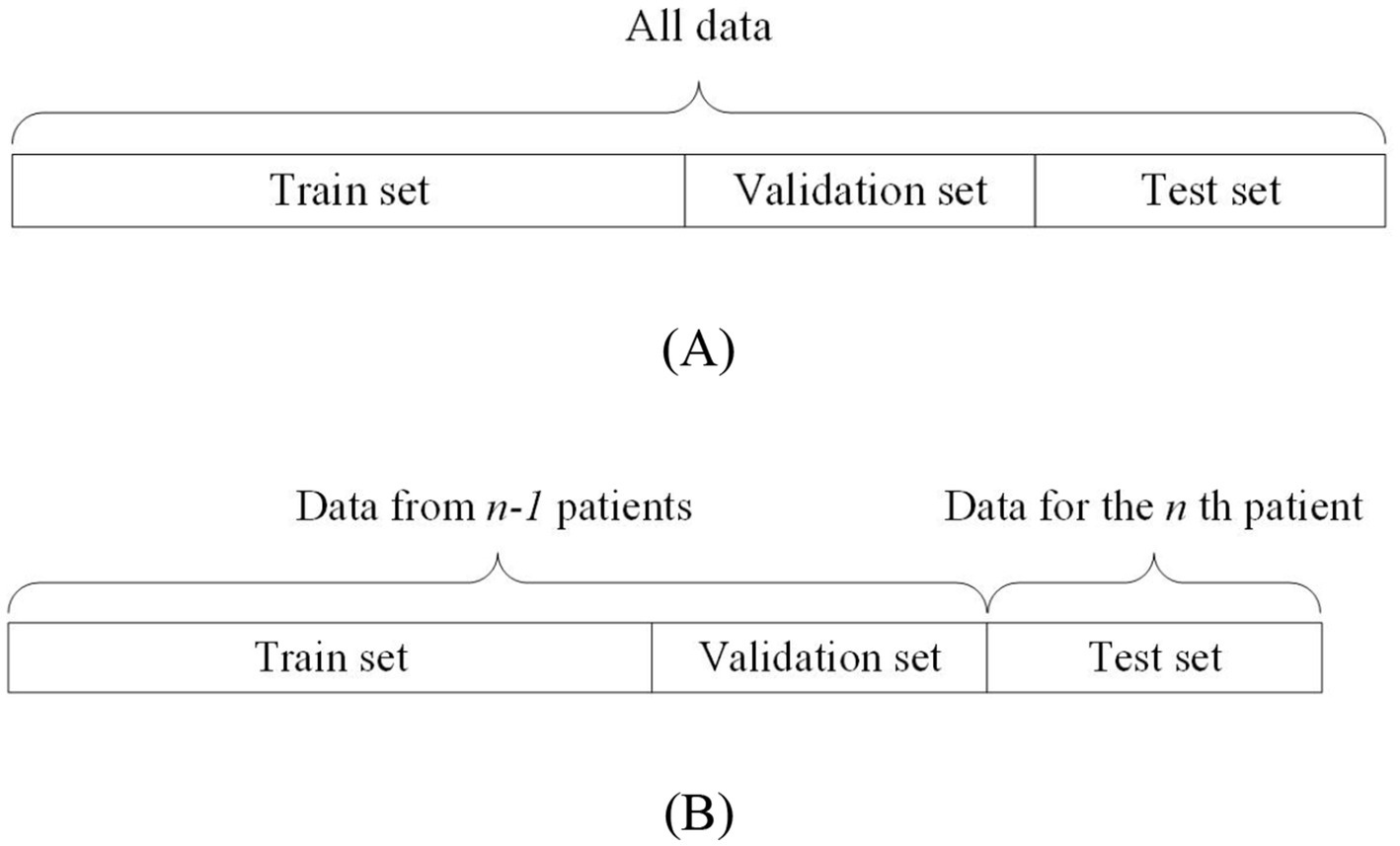
Figure 3. Schematic diagram of non-patient independent data segmentation.

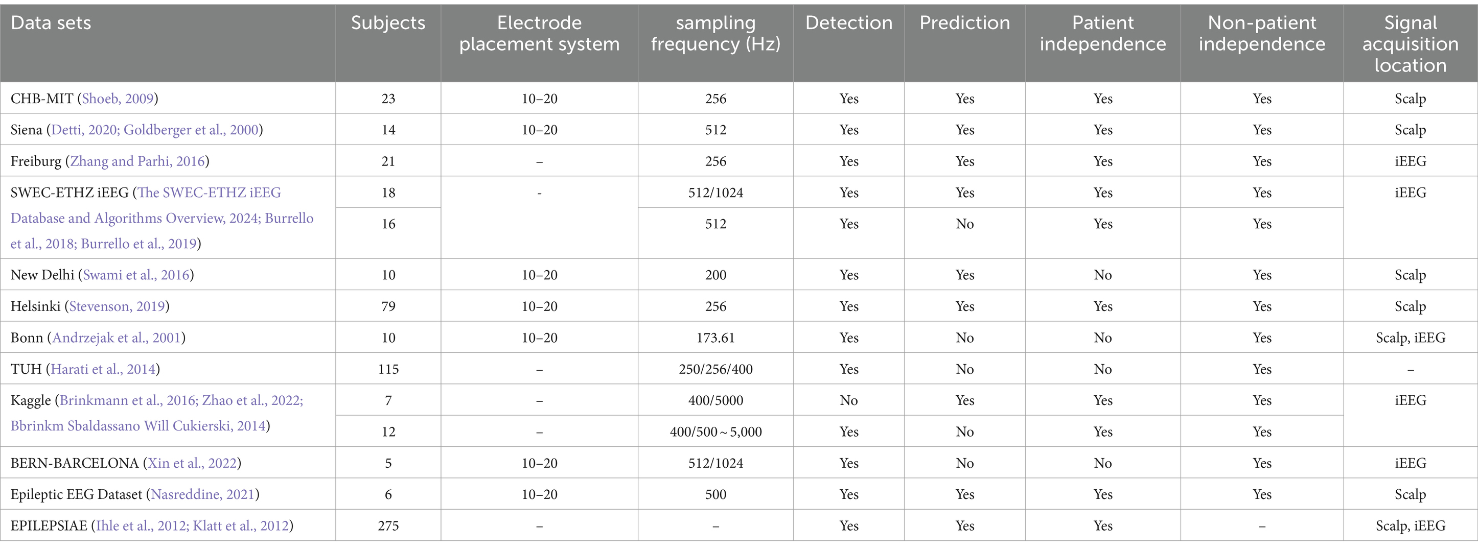
Table 1. Information on publicly available epileptic EEG datasets.

3 Techniques for pre-processing EEG signals in epilepsy

During EEG acquisition, artifacts such as electrocardiogram (ECG) signals, electromyogram (EMG) signals, and thermal noise can contaminate the data. Effective preprocessing of these artifacts is essential for improving the accuracy of epilepsy detection and prediction models. Several techniques are widely employed in the preprocessing of epileptic EEG signals, including thermal noise reduction, artifact removal, and data enhancement methods.

3.1 Thermal noise processing of EEG signals

Electromagnetic interference in the ambient environment and thermal noise inherent in the device can severely damage the low-amplitude EEG signal. The raw EEG signal is highly non-stationary and dynamic, and the scalp EEG itself is small in amplitude, so it is easily affected by high-frequency interferences as well as 50 Hz or 60 Hz signals (Lakehal and Ferdi, 2024; Wang et al., 2024). A 50 Hz or 60 Hz notch filter is commonly used to remove the industrial frequency noise (Raghu et al., 2020). High-frequency noise is filtered out using a high pass filter, low pass filter, band pass filter, etc (Liu et al., 2022).

3.2 Removal of artifacts in EEG signals

To address thermal noise and artifacts in EEG data, various signal processing methods have been developed. Techniques such as Wavelet Transform (WT), Empirical Mode Decomposition (EMD), and Blind Source Separation (BSS) are commonly employed to identify and remove these artifacts.

WT denoising works by using a basis function to compute the wavelet coefficient that represent the degree of similarity between the basis function and the original signal. Noise is removed by setting a threshold for these coefficients; those below the threshold are discarded, and the remaining coefficients are used to reconstruct the denoised signal. For example, Zhou et al. (2021) proposed a dynamic thresholding method based on Discrete Wavelet Transform (DWT) for artifact removal, which has proven effective in enhancing EEG signal quality. Similarly, Yedurkar and Metkar (2020) applied DWT with adaptive filtering to remove low-frequency physiological artifacts while retaining more useful signal components.

However, the basis function in wavelet denoising is set manually and lacks adaptability. This limitation can be addressed by EMD, which decomposes any complex signal into multiple Intrinsic Mode Functions (IMFs) at different frequencies. A denoised signal can be obtained by setting a threshold to discard inappropriate IMFs and reconstructing the remaining ones. Parija et al. (2020) processed EEG signals by selecting the first four high-frequency IMFs from EMD, although the selection criteria lack a strong theoretical basis. Moctezuma and Molinas (2020) further refined EMD by filtering out noisy IMFs using Minkowski distance, while Karabiber Cura et al. (2020) applied energy, correlation, and other statistical measures to screen suitable IMFs for both EMD and Ensemble Empirical Mode Decomposition (EEMD). Hassan et al. (2020) obtained clean EEG signals using Complete Ensemble Empirical Mode Decomposition with Adaptive Noise (CEEMDAN) and NIG parameters. Bari and Fattah (2020) concluded that extracting the first IMF components is the most desirable by comparing the amplitudes and frequencies of IMFs obtained after CEEMDAN decomposition. Variational Modal Decomposition (VMD) offers an alternative approach, solving the problem of mode mixing in EMD and reducing computational complexity, as demonstrated by Liu et al. (2022), who removed noise by correlating VMD functions with the original signal. Peng et al. (2021) proposed the Elastic Variational Mode Decomposition (EVMD) algorithm, which is able to capture the center frequency variations of EEG signals in various frequency band segments compared to VMD, thus improving the experimental performance.

However, EMD has limitations, including mode mixing, noise introduction, and high computational complexity. These drawbacks can be addressed by BSS. BSS operates on the principle that a signal can be represented as a linear combination of different source signals. By decomposing the signal into multiple source components, discarding the noisy ones, and reconstructing the remaining components, a denoised signal can be obtained. Classical BSS techniques include Canonical Correlation Analysis (CCA), Principal Component Analysis (PCA), and Independent Component Analysis (ICA). While CCA and PCA are effective for analyzing linear signals, ICA is better suited for nonlinear signals, making it a more commonly used method for artifact removal in EEG data. Islam et al. (2020) introduced an advanced ICA variant, Infomax ICA, which showed improved reliability in separating components based on mutual information. Becker et al. (2015) enhanced ICA with a penalized semialgebraic deflation algorithm, reducing computational complexity while maintaining performance. Beyond conventional approaches, several innovative methods have been developed for denoising epileptic EEG signals. Sardouie et al. (2014) introduced two semi-blind source separation techniques based on time-frequency analysis: Time-Frequency Generalized Eigenvalue Decomposition (TF-GEVD) and Time-Frequency Denoised Source Separation (TF-DSS). These methods were shown to outperform traditional techniques. Qiu et al. (2018) proposed the Denoising Sparse Autoencoder (DSAE), an advanced deep neural network that combines the strengths of sparse and denoising autoencoders. By enforcing sparsity in the hidden layers, this method efficiently represents EEG signals, particularly when dealing with non-smooth, noisy data. The DSAE’s ability to learn robust representations of the underlying EEG signals makes it a valuable tool for improving the accuracy of seizure detection. Lopes et al. (2021) explored a deep learning approach by developing a Deep Convolutional Neural Network (DCNN) model for artifact removal in EEG data. This model is particularly effective in handling nonlinear signal sources and removing various artifacts, including those caused by eye blinks, muscle activity, and channel motion. Despite its complexity, the DCNN model offers significant improvements in denoising performance.

However, BSS requires a reference waveform to effectively remove noise by linking it with multiple source signal waveforms. Recognizing that each denoising method has its strengths and limitations, researchers have also explored hybrid approaches to improve the purity of EEG signals. Du et al. (2024) employed a combination of CEEMDAN and Continuous Wavelet Transform (CWT) for joint denoising of epileptic EEG signals. This approach further improves signal quality by integrating the benefits of both CEEMDAN and CWT, offering a more comprehensive noise reduction strategy. Please refer to Table 2 for details.

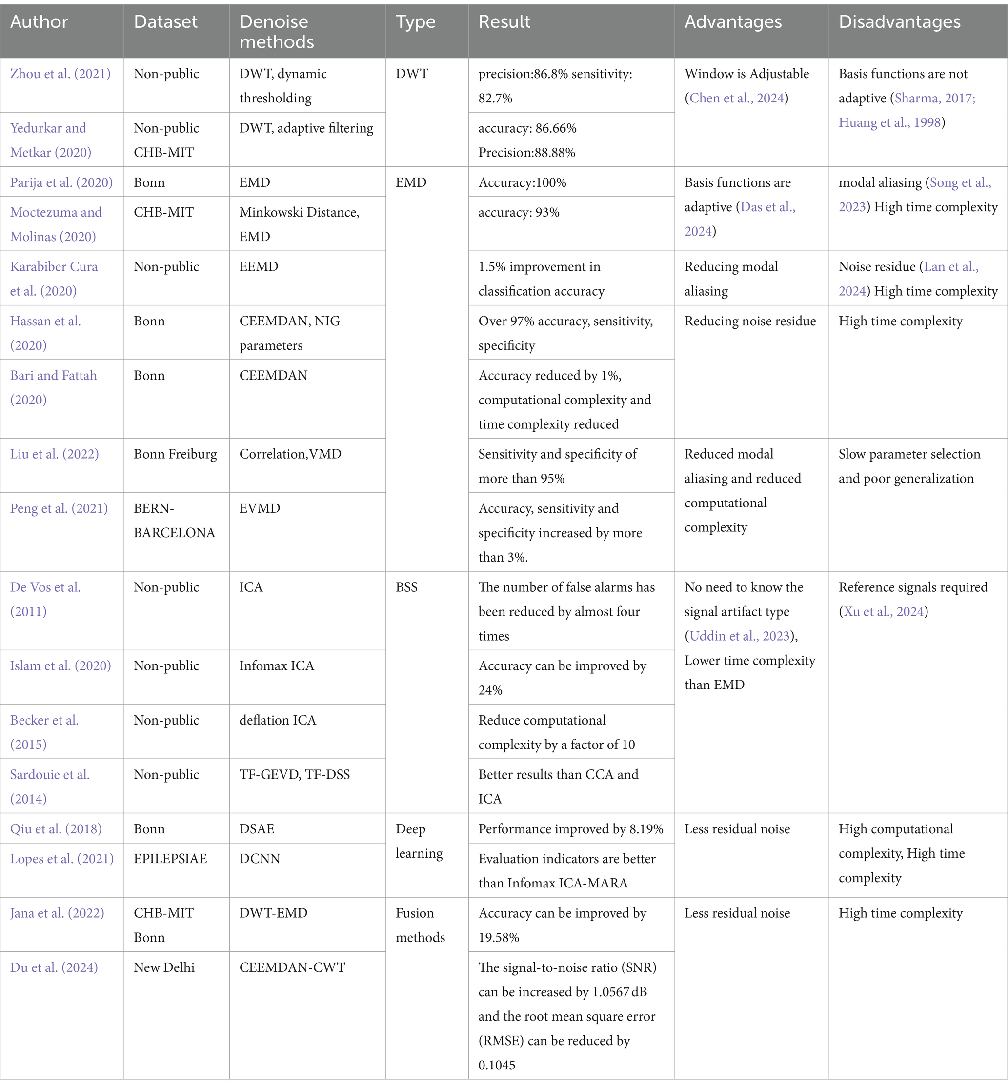
Table 2. Denoising methods for epileptic EEG signals.

3.3 Data enhancement

In addition to artifact removal, data enhancement techniques are crucial for improving the quality of EEG signals, especially when dealing with small or imbalanced datasets. Data augmentation methods, such as flipping, windowing, and adding noise, are commonly used to artificially expand datasets (Wan et al., 2023). Palanisamy and Rengaraj (2024) employed these techniques by increasing the amplitude and applying random transformations to EEG signals, thereby enhancing the robustness of deep learning models.

Generative Adversarial Networks (GANs) represent a more sophisticated approach to data augmentation. Initially proposed by Goodfellow et al. (2014), GANs generate synthetic data that can balance training datasets, as demonstrated by Gao et al. (2022) with their GAN-based model for seizure detection. Temporal Generative Adversarial Networks (TGAN) and Wasserstein Generative Adversarial Networks (WGANs) have also been employed to address temporal dependencies and gradient vanishing issues in EEG data, respectively. Nasiri and Clifford (2021) propose a Generative Transferable Adversarial Network (GTAN) that generates transferable adversarial features to address the performance degradation of traditional algorithms due to inter-individual variation in EEG data. A comparison of each method is shown in Table 3.

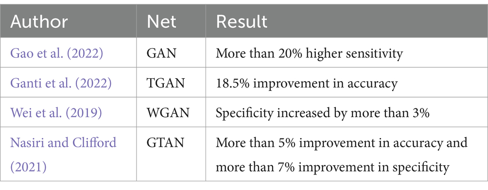
Table 3. A comparison of each method.

4 Feature extraction techniques for epileptic EEG signals

Feature extraction can streamline and organize underlying patterns, making them more manageable. Although neural networks are capable of automatically identifying useful features from raw data, well-engineered features can simplify problem-solving. This approach often requires less data and fewer resources to achieve effective results (Francois, 2022). Feature extraction in EEG signal analysis involves time-domain features, frequency-domain features, time-frequency domain features, and nonlinear dynamics features. Time-domain features provide a general overview of the signal’s distribution but do not capture frequency-related information. Conversely, frequency-domain features convert signals from the time domain to the frequency domain, enabling the extraction of frequency-specific information. Time-frequency domain methods offer a more nuanced approach by representing spectral signals over time, combining both temporal and spectral analyses (Pham, 2021; Qin et al., 2024). Nonlinear dynamics, on the other hand, are used to quantify the chaotic nature of EEG signals, offering insights into their complexity (Yan et al., 2022).

Sun and Chen (2022) utilized entropy-based features, such as Sample Entropy (SampEn), Permutation Entropy (PermEn), and Fuzzy Entropy (FuzzyEn), both individually and in combination, to form three-dimensional feature vectors. Their findings indicated that combining SampEn, PermEn, and FuzzyEn produced the highest accuracy and recall rates. However, this approach did not incorporate time or frequency domain information. Fei et al. (2017) addressed this limitation by employing the Fractional Fourier Transform (FrFT), the adaptive maximal Lyapunov exponent, and its energy, which captured both the chaotic and frequency domain characteristics of epileptic EEG signals. Wang et al. (2019) Extracting features of the signal using Teager energy entropy, curve length and Teager-Huang transform results in better results than ordinary energy entropy. Zhang et al. (2024) took a more comprehensive approach by extracting features using DWT, Power Spectral Density (PSD), standard deviation, band energy, and FuzzyEn. While this method effectively gathered diverse feature information, it also introduced redundancy and increased computational complexity. To mitigate these issues, Zhang et al. (2018) generated 2,794 features for each sample using multiple feature extraction methods. These features were evaluated by a series of three consecutive selection algorithms, i.e., VarA, iRFE, and BackFS, to screen important features. Table 4 presents a summary of various feature extraction methods employed in the analysis of epileptic EEG signals.

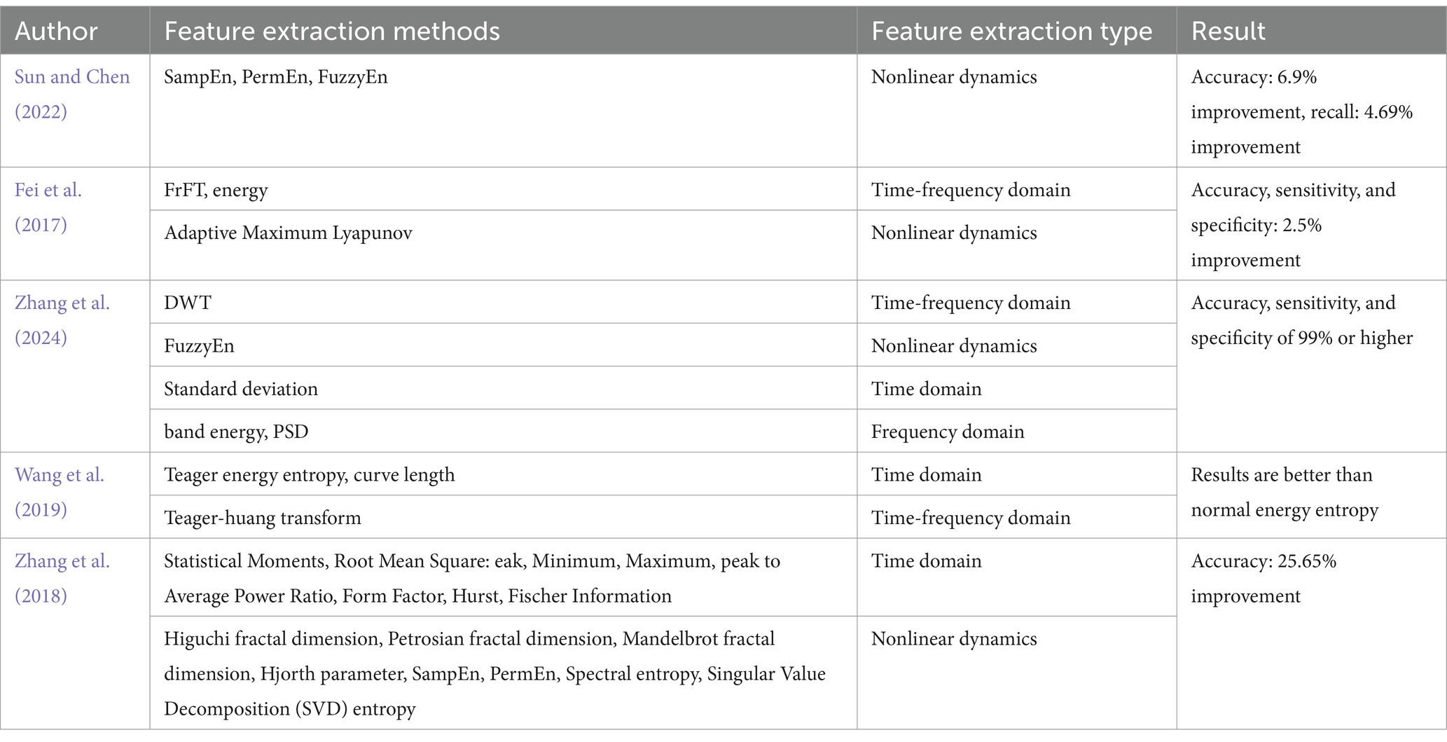
Table 4. Feature extraction methods for epileptic EEG signals.

5 Algorithms for detection and prediction of epileptic EEG signals

After preprocessing and feature extraction on the data, the processed signal is then fed into the network model for deep feature extraction and classification.

5.1 Assessment of indicators

In evaluating deep learning models for epileptic EEG signal detection and prediction, specific assessment metrics are employed to measure performance effectively.

For seizure detection, the evaluation is typically straightforward, relying on standard classification metrics such as Accuracy, Sensitivity, Specificity, Precision, F1 Score, Receiver Operating Characteristic (ROC) curve, Area Under the ROC Curve (AUC), and False Positive Rate (FPR). These metrics provide a clear measure of how well the model distinguishes between seizure and non-seizure events.

In contrast, seizure prediction models are designed to differentiate between inter-ictal (periods between seizures) and pre-ictal (periods just before a seizure) states, which requires a more nuanced approach. While prediction models often use the same metrics as detection models, a specialized set of criteria—known as the Epilepsy Prediction Evaluation Criteria—was introduced by Maiwald et al. (2004). This method includes several key metrics: Maximum False Positive Rate (FPRmax): The highest allowable prediction error rate within a given time interval. Seizure Onset Period (SOP): The timeframe during which a seizure is expected to occur following a prediction. Seizure Prediction Horizon (SPH): The time interval between the prediction and the SOP. Figure 4 provides a schematic representation of SPH and SOP.

Figure 4. Schematic diagram of SPH and SOP concepts.

The process for applying these criteria begins with setting initial values for FPRmax, SPH, and SOP. The model’s parameters are then adjusted to ensure that the false prediction rate for each patient remains within the set FPRmax. The sensitivity for each patient is calculated, and the average sensitivity across all patients is determined. This process is repeated iteratively to establish reasonable ranges for FPRmax, SPH, and SOP, as shown in Figure 5. This methodology builds on earlier work by Osorio et al. (1998), who emphasized the importance of considering both FPR and sensitivity in prediction models. Notably, there is a trade-off between the FPR and sensitivity.

Figure 5. Flowchart for determining FPRmax, SPH and SOP.

5.2 Convolutional neural networks

CNNs, first introduced in 1980, can learn both feature extraction and classification layers within the network. This dual learning enhances the network’s generalization ability, making CNNs particularly effective for processing complex signals (Hassan et al., 2024). Given the non-linear and intricate nature of EEG signals, CNNs are well-suited for their analysis (Hassan et al., 2024). CNNs are structured with several key components: an input layer, convolutional layers, pooling layers, fully connected layers, and an output layer. The convolutional layers, equipped with convolutional kernels, are crucial for extracting features from the input data. Pooling layers further compress the feature space, which reduces computational complexity. The fully connected layers consolidate these features and serve as classifiers. This architecture allows CNNs to be both efficient in computation and effective in training due to the localized and globally shared connections between neurons in the convolutional layers. Figure 6 shows the Diagram of CNN.

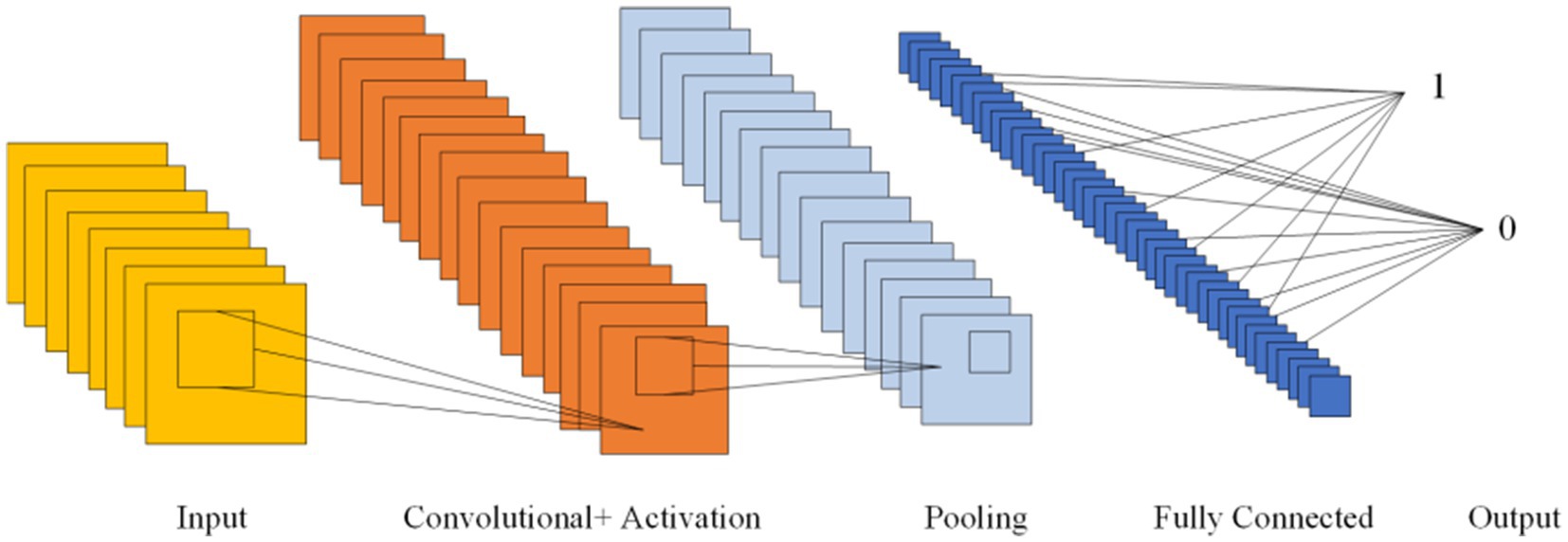
Figure 6. Diagram of CNN.

Several studies have explored CNNs for epilepsy detection. Acharya et al. (2018) introduced a 1-Dimensional Convolutional Neural Network (1D-CNN) that directly classifies EEG signals without prior feature extraction. Their approach achieved an average accuracy of 88.7%, with a sensitivity of 95% and specificity of 90%. In contrast, Wang et al. (2021) used a stacked 1D-CNN on two public datasets, also skipping pre-processing and feature extraction. Their results demonstrated high accuracy and specificity (over 99%), but the absence of a test set leaves their findings open to debate. Avcu et al. (2019) utilized a 2-Dimensional Convolutional Neural Network (2D-CNN) with only two channels of data, outperforming models that used 18 channels. Das et al. (2024) compared 1D-CNN and 2D-CNN by reshaping data into both formats, finding that the 2D-CNN offered superior classification performance. Pan et al. (2022) proposed a lightweight 2D-CNN that processed both raw data and data transformed by various techniques, such as Discrete Fourier Transform (DFT), Short-Time Fourier Transform (STFT), DWT. While this hybrid method improved detection performance with limited data, the lack of a test set data raised concerns about model reliability. Xu et al. (2024) introduced a 3-Dimensional Convolutional Neural Network (3D-CNN) aimed at reducing the latency of seizure detection through probabilistic prediction, achieving detection delays at least 50% shorter than previously reported.

Table 5 lists various epilepsy detection models based on CNNs, detailing their accuracy (Acc), sensitivity (Sen), and specificity (Spe). The table also indicates the data partitioning methods used, with #1 indicating a segment-based data partitioning approach, #2 indicating an event-based data partitioning approach, *1 indicating an all-patient-based data partitioning approach. If the symbols (#1,#2,*1) are not indicated, it means that the method of partitioning the dataset is not applicable or not specified in the article.

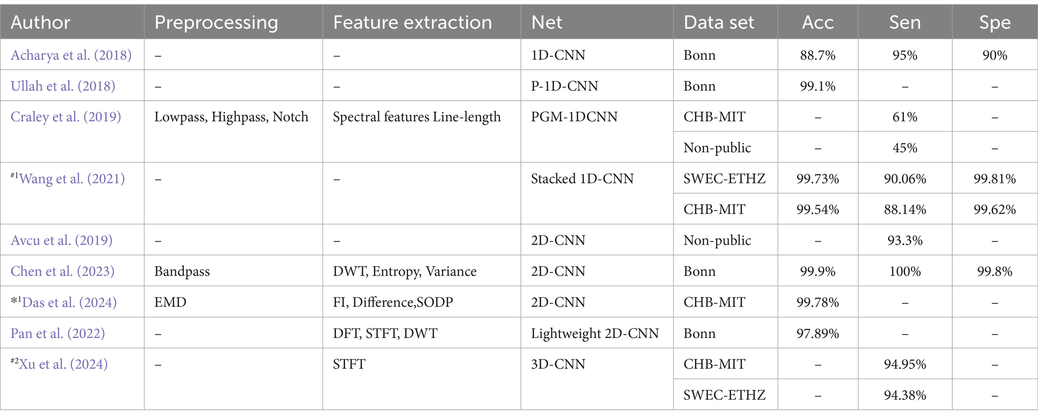
Table 5. Epilepsy detection model based on convolutional neural network.

CNNs prediction based on metrics of common classification methods: Shafiezadeh et al. (2024) introduced a calibration pipeline using a 2D-CNN model. By incorporating a small amount of data from test set patients into the training set, their approach fine-tunes the model to predict epileptic events from new patients. This method improved accuracy, sensitivity, and specificity by over 15% on the CHB-MIT dataset and by more than 19% on a non-public dataset. But the computational complexity is too high. Zhang et al. (2021) Proposed Lightweight-2D-CNN reduces computational complexity.

Table 6 outlines various CNNs prediction models and their performance metrics, including accuracy (Acc), sensitivity (Sen), specificity (Spe), and pre-epileptic time (PT) in minutes. It also denotes data partitioning methods: #2 indicating an event-based data partitioning approach, *1 indicating an all-patient-based data partitioning approach, and *2 indicating a cross-patient data partitioning approach. * indicates that the article only describes how the data are divided for non-independent patients and does not mention a specific way of partitioning the data. If the symbols (#2,*1,*2,*) are not indicated, it means that the method of partitioning the dataset is not applicable or not specified in the article.

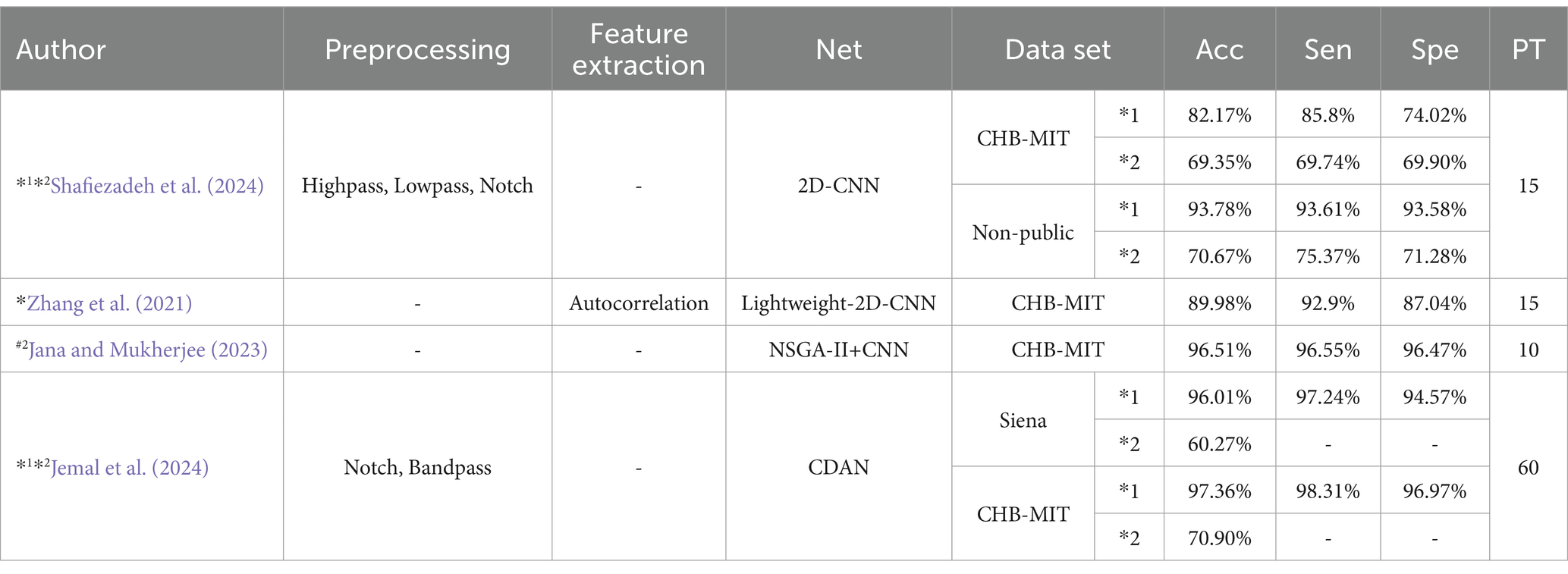
Table 6. CNN prediction model based on common classification method metrics.

CNNs prediction model based on evaluation criteria for epilepsy prediction: Truong et al. (2018) proposed a 2D-CNN model tested on both scalp and intracranial EEG data. Their model achieved a sensitivity greater than 89% across both datasets, though the Freiburg dataset exhibited a higher FPR. Ra and Li (2023) utilized Simultaneous Extractive Transform (SET) and Singular Value Decomposition (SET-SVD) to enhance time-frequency resolution, achieving a sensitivity over 99.7% with a 1D-CNN model. Ozcan and Erturk (2019) explored spatiotemporal correlations in EEG signals using a 3D-CNN, which showed an 85.7% sensitivity and an FPR of 0.096/h on the CHB-MIT dataset. To improve interpretability: Prathaban and Balasubramanian (2021) developed a dynamic learning framework with a 3D-CNN model optimized by the Fletcher Reeves algorithm. Their phase-transform-based method demonstrated precise real-time seizure prediction using scalp EEG data.

Table 7 presents CNN prediction models based on evaluation criteria such as sensitivity (Sen), FPR, SOP, and SPH, all measured in minutes. It also denotes data partitioning methods: # indicates that the article only describes how the data are divided for independent patients and does not mention a specific way of partitioning the data. If the # is not indicated, it means that the method of partitioning the dataset is not applicable or not specified in the article.

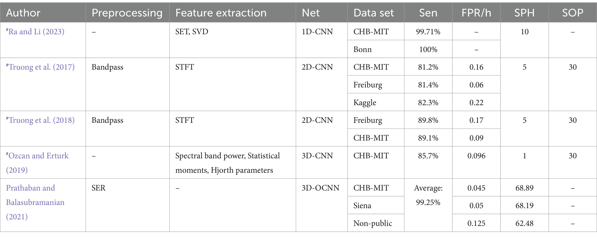
Table 7. CNN prediction model based on evaluation criteria for epilepsy prediction.

5.3 Recurrent neural networks

RNNs are designed to process time series data and consist of an input, hidden, and output layer. Unlike CNNs, RNNs allow neurons to receive information not only from other neurons but also from themselves, creating a network with loops. This loop structure enables RNNs to maintain a memory of previous inputs through hidden units, making them particularly suitable for processing EEG data. Figure 7 illustrates the structure of an RNN, where ht represents the hidden state at time t, and the delay mechanism records the most recent hidden state. However, RNNs often struggle with the issue of vanishing gradients, which is mitigated by LSTM and GRU.

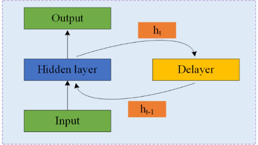
Figure 7. Structure and schematic diagram of RNNs.

LSTM networks address this issue by using input and forget gates to manage memory. As shown in Figure 8A, LSTM cells use the external state ht − 1 at time t − 1 and the input xt at time tt to calculate the forget gate ft, input gate it, output gate ot, and candidate state ĉt. These elements are then combined with the memory unit ct − 1 to update the memory unit ct at time tt. Finally, the external state ht at time tt is derived from the memory unit ct and the output gate ot. While the complementary relationship between the forget and input gates enhances the LSTM’s memory management, it also introduces some redundancy.

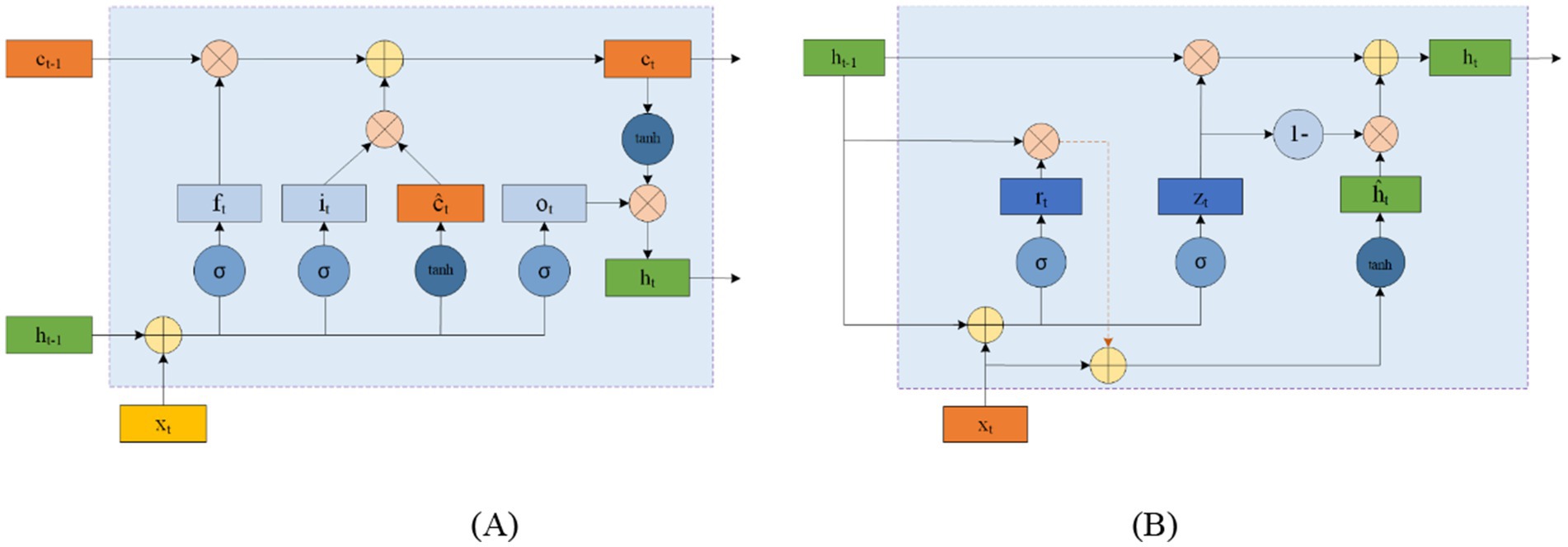
Figure 8. Circular unit structure of LSTMs (A) and GRUs (B).

GRU offers a simpler alternative to LSTM by consolidating the input and forget functions into a single gate. Figure 8B shows the structure of a GRU cell, where the reset gate rt controls the influence of the previous state ht − 1 on the candidate state ĥt. The update gate zt regulates the balance between retaining information from the historical state and incorporating new information from the candidate state. xt represents the input at time tt, and ht is the resulting state.

For epilepsy detection using RNNs, Hu et al. (2020) proposed a Bi-directional Long Short-Term Memory Network (Bi-LSTM) that classifies EEG data using 11 time-domain features extracted through Local Mean Decomposition (LMD). Their method achieved an average sensitivity of 93.61% and specificity of 91.85%. Zhang et al. (2022) also employed a Bi-directional Gated Recurrent Unit (Bi-GRU) for epilepsy detection. They utilized DWT and wavelet energy features, achieving an average sensitivity of 93% and specificity of 98.49%. Tuncer and Bolat (2022) used only instantaneous frequency and spectral entropy features with a Bi-LSTM network, obtaining an average classification accuracy of 97.78%, surpassing Hu’s results but using the Bonn dataset.

In terms of epilepsy prediction, Singh and Malhotra (2022) used a Two-Layer Long Short-Term Memory Network (2 L-LSTM), incorporating Fast Fourier Transform (FFT), spectral power, and mean spectral amplitude for feature extraction. Tsiouris et al. (2018) employed a range of features, including statistical moments, time-domain features, and various transforms (FFT, SD, DWT), within a 2 L-LSTM framework. Their approach demonstrated sensitivity and specificity greater than 99%, outperforming Kuldeep’s results.

5.4 Generating adversarial networks

GANs were proposed by Goodfellow et al. (2020). GANs consist of two components: a generator and a discriminator. The generator creates synthetic data, which is then evaluated by the discriminator to determine its authenticity. Feedback from the discriminator helps both components improve their performance. The structure of GANs is shown in Figure 9. Some of the epileptic EEG datasets have less amount of data, e.g., New Delhi dataset, Bonn dataset, this situation leads to poor learning ability of the network and risk of overfitting. GANs are capable of generating simulated data that is very similar to the real data compared to the other data enhancement methods, which improves the performance of the model. GANs have recently been explored for epilepsy classification tasks.

Figure 9. Structure of GANs.

Truong et al. (2019) were among the first to apply GANs to seizure prediction. They used a Deep Convolutional Generative Adversarial Network (DCGAN) to learn features from Time-Frequency domain signals processed with STFT. Despite their innovative approach, DCGAN is known for issues with gradient vanishing and instability (Fathallah et al., 2023).

5.5 Transfer learning

Transfer learning can be traced back to the late 20th century and the early 21st century (Burrello et al., 2019; Pan and Yang, 2009). Transfer learning is the use of knowledge gained from one task to improve performance on a related task. First, a basic network is trained on the source dataset and task, and then the learned features (network weights) are applied to a new network trained on a different but related dataset and task. This approach helps to address the problem of EEG data scarcity, and compared to other network models, transfer learning can reduce the resources and time required to train deep learning models (Yang et al., 2024; Weiss et al., 2016; Butt et al., 2024)

In the context of epilepsy detection and prediction, Liang et al. (2020) utilized a combination of the Visual Geometry Group network (VGG) and LSTM for analyzing EEG signals. Their method demonstrated strong results through cross-validation, though sensitivity for some patients was as low as 60%. Gao et al. (2020) employed three deep convolutional neural networks—Inception-ResNet-v2 (Inception Residual Network Version 2), Inception-v3 Network (Inception-v3), and Residual Network 152 (ResNet152)—to classify EEG data into various categories: interictal, reictal I, reictal II, and postictal. They set preictal I and II durations to 30 min and 10 min, respectively, to assess the importance of event duration. Takahashi et al. (2020) proposed an Autoencoder-assisted VGG Network (AE-VGG-16) for seizure detection, which significantly reduced FPR. Toraman (2020) compared three pre-trained CNN models: VGG16, Residual Network (ResNet), and Densely Connected Network (DenseNet)—using spectrogram images to differentiate between pre-seizure and inter-seizure states. The study found that the ResNet model provided the best performance.

5.6 Fusion model

Fusion modeling combines different network types to leverage their strengths and mitigate their weaknesses. This approach enhances model performance by integrating various methodologies. Transformers and Residual blocks are commonly used in fusion models. The Transformer was first proposed in 2014 by Bahdanau (2014). A Transformer Network includes an input layer, encoder, decoder, and output layer, with a multi-head attention mechanism added between the encoder and decoder (Wang et al., 2024; Zhang et al., 2024a; Cho et al., 2014). This mechanism effectively manages the performance of the model as EEG sequence length increases and improves processing efficiency for long sequences, thus reducing time complexity (De Santana Correia and Colombini, 2022; Rukhsar and Tiwari, 2023). Figure 10A shows the Transformer structure. The ResNet was introduced in 2015 by He et al. (2016). The residual block helps to retain the data from the previous layers and solve problems such as overfitting of the EEG signal on other networks and gradient vanishing. Figure 10B shows the residual block structure.

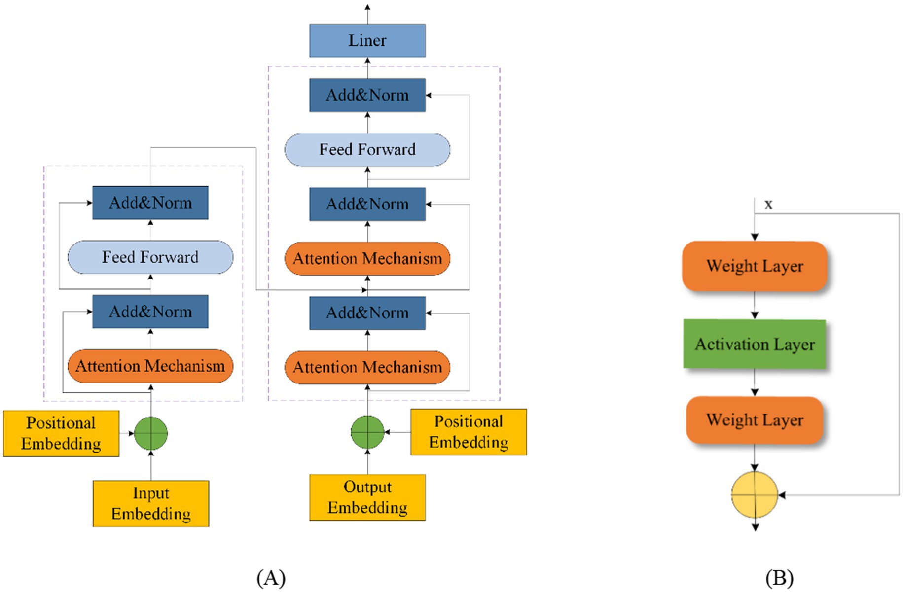
Figure 10. Transformer structure (A) and residual block structure (B).

In the field of epilepsy detection, Sunaryono et al. (2022) introduced a hybrid model combining a 1D-CNN with majority voting and Deep Neural Networks (DNNs). This method achieved 100% accuracy in detecting epilepsy from EEG signals, though its effectiveness may vary with datasets other than the University of Bonn dataset. Awais et al. (2024) proposed a Graph Convolutional Neural Network-Long Short-Term Memory Network (GCN-LSTM), which takes into account the spatial aspects of EEG signals. Huang et al. (2024) developed a Temporal Convolutional Neural Network with a Self-Attention (TCN-SA) layer to extract crucial features using self-attention. Zhu et al. (2024) introduced a Squeeze-and-Excitation Temporal Convolutional Network with Bidirectional Gated Recurrent Units (SE-TCN-Bi-GRU) that automatically selects important EEG channels, though it involves multiple parameters. Zhou et al. (2024) proposed a Lightweight Multi-Attention EEG Network (LMA-EEGNet) that reduces parameter count and network complexity while maintaining effective feature extraction.

Table 8 summarizes various detection algorithms based on hybrid models, detailing their accuracy (Acc), sensitivity (Sen), and specificity (Spe). Data partitioning methods are indicated, with #1 indicating a segment-based data partitioning approach, #2 indicating an event-based data partitioning approach, *2 indicating a cross-patient data partitioning approach. # indicates that the article only describes how the data are divided for independent patients and does not mention a specific way of partitioning the data; * indicates that the article only describes how the data are divided for non-independent patients and does not mention a specifi