1 Introduction

During concentrated learning of live or recorded lectures, the human mind is prone to turning inwards. This inherent mental process is often referred to as mind-wandering (MW). Generally, MW is defined by attention oriented away from an external task toward our internal, self-generated thoughts (Dong et al., 2021). Extended periods of MW correlate negatively with direct educational outcomes, manifesting as decreased information retention and comprehension (Risko et al., 2012; Szpunar et al., 2014). Additionally, MW may indirectly affect learning outcomes, potentially impairing note-taking abilities (Lindquist and McLean, 2011). However, our current understanding of the neural mechanisms of MW remains incomplete, and there is a lack of reliable and objective methods to accurately detect it (Dhindsa et al., 2019), which are critical for the development of strategies to mitigate the negative impact of MW.

In MW detection, task-related assessments (Zhang and Kumada, 2018) and physiological measures such as eye movement, pupillometry (Faber et al., 2018), heart rate, skin conductance, and synchronization between respiration and sensory pressure (Zheng et al., 2019) are commonly-used. Neural measures, including functional magnetic resonance imaging (fMRI) and electroencephalography (EEG), provide direct insights into this mental state (Dong et al., 2021). FMRI offers detailed spatial resolution, but with low temporal precision. Conversely, EEG captures brain activity at high temporal resolution and is cost-effective and wearable, but lacks the spatial accuracy of fMRI, especially for deep brain sources.

Recent studies have focused on using event-related potentials and spectral features to classify MW. A sustained attention task showed decreased P300 amplitude during MW (Smallwood et al., 2008), and other experimental studies support the idea that MW reduces cognitive resources for task processing (Kam and Handy, 2013; Kam et al., 2012; O'Connell et al., 2009). An experiment focusing on mindful breathing revealed lower occipital alpha and fronto-lateral beta power during MW compared to breath focus (Braboszcz and Delorme, 2011). Similar conclusions have been found in another study (van Son et al., 2019). Functional connectivity is an important feature in studying MW. Investigations using fMRI on MW suggest that it is associated with the default mode network (DMN) and the executive control network. The DMN is composed of brain regions that remain activation during rest and is linked to MW (Mason et al., 2007). A study found DMN to be active during self-reported instances of MW (Mooneyham and Schooler, 2013). However, DMN also exhibits heightened activity during purposeful internal thought, including future planning and episodic memory retrieval (Spreng et al., 2009; Buckner et al., 2008; Andrews-Hanna, 2012). This means activation of the DMN is not a specific indicator of MW.

MW is a highly dynamic process characterized by rapid fluctuations and spontaneity in thought, but the corresponding changes in functional connectivity networks over time are often overlooked (Konjedi and Maleeh, 2021; Christoff et al., 2016). Considering the dynamics during MW is thus crucial for better understanding and detection. Compared to fMRI, EEG offers higher temporal resolution, enabling better capture of the dynamical aspects of brain functional connectivity. However, to our knowledge, there is currently no EEG functional connectivity analysis for MW (Kam et al., 2022). Traditional brain network analysis often overlooks critical information, such as frequency or time domain relationships. Multilayer networks can integrate multiple data sources, capturing connectivity across different frequency bands, time scales, and variations in connectivity during different tasks. For example, in epilepsy, multilayer EEG networks revealed less variable activity during absence seizures (Leitgeb et al., 2020). In stroke, they showed reduced global connectivity and robustness (Hao et al., 2024); while in Alzheimer's disease, multiplex networks indicated disrupted brain activity and achieved high classification accuracy (Cai et al., 2020). A time-window-based multilayer model also enhanced understanding of brain dynamics during driving (Chang et al., 2022). These examples highlight how multilayer networks improve insights into brain function and cognition. Considering the above, our study will analyze the dynamic characteristics of multilayer functional connectivity networks built from EEG during MW.

In this study, we developed a multilayer network analysis framework that integrates different functional connection definitions, with network nodes representing electrodes. To sidestep the difficulties associated with selecting window size and sliding step size in traditional sliding window data segmentation methods (Xu et al., 2023), we improved our previous segmentation algorithm to apply it to multilayer networks. Our multilayer network features two layers: one using amplitude envelope correlation (AEC) for intra-layer edge weights and the other employing imaginary phase-locking value (IPLV) for intra-layer edge weights. In this study we used only two layers, but our method is scalable to more layers. The network is a weighted undirected multiplex network for each time segment. Quantified by overlapping node closeness centrality vectors, we clustered these networks into four states, each representing a recurring motif, and discretized EEG segments into time series of network state labels. Finally, we implemented a hidden Markov model to classify presence of MW based on these state sequences, assessing the effectiveness of our multilayer analysis.

The remainder of the article is organized as follows. We present a detailed description of the proposed method in Section. 2. We present results in Section 3. Finally, we discuss our work in Section 4 and conclude in Section 5.

2 Method 2.1 EEG data and pre-processing 2.1.1 Dataset

In this work, we conducted a detailed analysis of our EEG dataset that has been previously published (Tang et al., 2023). For more comprehensive methodological details, see that article; a brief summary is below.

2.1.2 Participants and task design

A total of 14 healthy participants (six females and eight males; average age 23.36 ± 4.75 years) were engaged in the study. The two distinct experimental conditions were: the focused learning (FL) condition, during which the two most highly-rated (for interest) lecture videos chosen by each participant was shown to him or her; and the future planning condition, during which the two least interesting videos were shown. In the future planning condition, in which participants engaged in personal future planning cued by images (previously collected from them) displayed on screen before the lecture video. Following each video, participants provided feedback through rating scales, assessing their estimates of percentage of time focused on the video and percentage of time in intentional and unintentional mind-wandering. In this study, the mental state during the future planning condition is assumed to be MW (and called the MW condition hereafter), while that in the FL condition is assumed to be non-MW. During the video, participants could press a key to indicate deviation from the task in each condition, data thus marked are not analyzed here.

2.1.3 EEG acquisition and pre-processing

The EEG data analyzed here were collected using an 8-channel system (Yiwu Jielian Electronic Technology Co., Ltd, China) at a sampling rate of 1,000 Hz. The low channel count was intended to make the system more easily deployable. Electrodes were positioned at F3, F4, T3, C3, C4, T4, O1, and O2 according to the International 10-20 EEG system, with the reference electrode at CZ. The raw data underwent high-pass filtering at 1 Hz, down-sampling to 256 Hz, and notch filtering at 48–52 Hz. To mitigate noise interference, we implemented artifact subspace reconstruction (ASR) using the clean raw data plugin of EEGLab. Pre-task resting-state signals served as calibration data, with artifacts being either removed or corrected based on specific parameters (“BurstCriterion”=30 and “WindowCriterion” = 0.3) (Kothe and Jung, 2016). Additionally, we employed an amplitude threshold-based method to further detect and eliminate noise-contaminated time segments. Subsequently, EEG signals were band-pass filtered into delta (1–4 Hz), theta (4–8 Hz), alpha (8–13 Hz), beta (13–30 Hz), and gamma (30–80 Hz) frequency bands using windowed-Hamming finite impulse response filters, using the default filtering method and settings of MNE-Python (Gramfort et al., 2013).

2.2 Multilayer network construction 2.2.1 Design of multilayer networks

In this study, we construct weighted multilayer networks which integrate two types of functional connectivity. Taking a segment of EEG data as an example (see Figure 1A), we assessed the functional connectivity between each pair of EEG channels using AEC and separately IPLV. Thus, two 8 × 8 connectivity matrices are obtained, as illustrated in Figure 1B. We construct a two-layer weighted network (see Figure 1C), where nodes of the network correspond to channels.

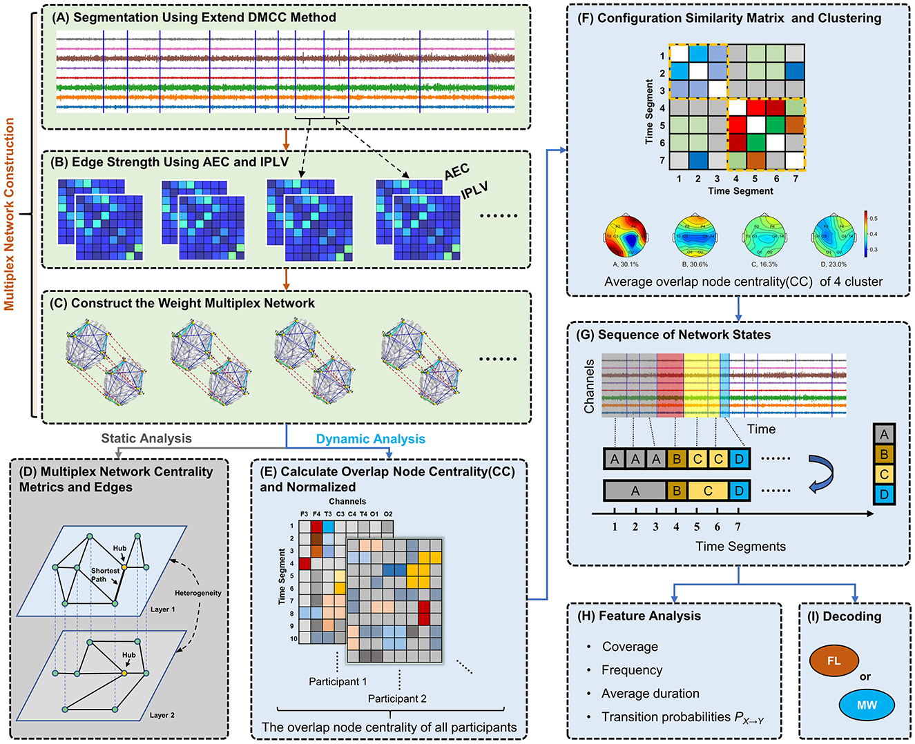
Figure 1. Diagram of analytical methods. (A) Segmentation of 8-channel EEG data based on changes in network structure. (B) Construction of functional connectivity networks for each segment using AEC and IPLV for the first and second layer, respectively. (C) Weighted multiplex networks are formed. Connection thickness in visualization indicates edge weight. (D) Analysis of static network topology (one segment). (E) Calculation of overlap node closeness centrality for each node. (F) Clustering of networks (segments) by their node centrality vectors using the Louvain algorithm, producing clusters representing typical recurring network states. (G) Discretization of EEG data into a network state sequence based on clustering results. (H) Computing and analysis of various dynamical features (statistics of state sequences). (I) Classification of network state sequences as mind-wandering or focused learning via a hidden Markov model.

The edge weights in the first layer are determined by AEC. The computational procedure for AEC is delineated by the following rules (Bruns et al., 2000; Zamm et al., 2018): amplitude envelopes were generated via Hilbert transform of the EEG data in the segment; Pearson correlations were then computed between all amplitude envelopes across all combinations of channel pairs. Finally, we calculated the absolute values of the correlation coefficients to prevent cancellations during averaging, as envelope correlations can be negative. Additionally, negative values lack practical significance in brain network analysis for our purposes.

Considering that the edges in the first layer are calculated from the perspective of amplitude, to minimize overlap with the information of the first layer, we chose IPLV to measure functional connectivity strength in the second layer. The calculation of IPLV is as follows (Sadaghiani et al., 2012):

IPLV=1N∣Im(∑n=1Nexp[i(ϕchannel1(n)-ϕchannel2(n))])∣,    (1)

where N is the total number of time points within an EEG data segment, and ∣·∣ denotes the complex modulus. The Hilbert transformation is used to calculate the analytic phase at time point n as ϕchannel_j(n) = arctan[u(n)/v(n)], where v is the real part of the analytic signal, u is the Hilbert transform or the imaginary part Im(·) of the analytic signal.

The two crucial questions for constructing multilayer networks are: (1) whether there are differences between interlayer and intralayer connections; (2) whether different layers hold distinct meaning. We set a one-to-one correspondence between nodes in different layers based on the position of EEG channels, and interlayer connections exclusively link a node to its corresponding node in the other layer. This type of multilayer network is also known as a weighted multiplex network (Boccaletti et al., 2014). The interlayer edge weights are unconstrained, that is, there is no traversal cost associated with interlayer edges. Considering the possibility of different scales for edge weights between layers, we normalize each edge ei of the layer i in our multilayer network as follows:

ei=ei-rmin,irmax,i-rmin,i,    (2)

where rmin, i and rmax, i represent the minimum and maximum values e of the edges of layer i.

2.2.2 EEG segmentation

To avoid an EEG data segment containing more than one network motif, we segmented EEG based on network structure using the DMCC (distance measure/closeness centrality) variant of our previously published segmentation method (Xu et al., 2023). Our method was previously designed for single-layer networks, thus we here improve the method by comparing each layer between time windows, and we call the new variant the extend DMCC (EDMCC). Given two time periods T1 and T2, the extended procedure computes the following distance measure:

d(C(T1),C(T2))=∑i=1n(1m∑l=1mci[l](T1)-1m∑l=1mci[l](T2))2,    (3)

where n is the number of channels. m denotes the number of the network layers. ci[l](T1) denotes the closeness centrality of the node i in the layer l of multilayer network G(T1). C(T1) is a matrix of size n×m, consisting of the node centralities of each node of each layer. The most sensitive parameters of the segmentation algorithm were set thusly: reference window length Wr = 2s, probability of outlier selection pKDE = 0.96. Other parameter settings are the same as in our previous work (Xu et al., 2023).

Using this method, the EEG data were divided into segments of varying lengths (delta: 1.95 ± 0.835, theta: 1.998 ± 0.888, alpha: 2.07 ± 0.951, beta: 1.984 ± 0.843, gamma: 1.995 ± 0.859; average ± standard deviation seconds per segment). Compared with sliding windows of the same length (2 s for all bands), EDMCC performs better (see Figure 2A) in terms of an index that measures the difference in structure between segments compared to within segments [details on this pdiff index can be found in Xu et al. (2023)].

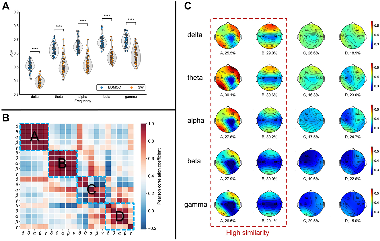
Figure 2. (A) Segmentation performance as measured with pdiff (higher values are better) for different frequency bands. EDMCC is an extension of our previous segmentation method to multilayer networks. SW denotes segmentation into same-length sliding windows. Each data point is the pdiff value of a block of EEG data in a frequency band. ****p < 0.0001. (B) Correlation of multilayer network states across states (ABCD) and frequency bands. (C) Average overlapping node closeness centrality of the multilayer networks for each multilayer network state (column). Numerical values under the topographic maps denote the ratio of total time spent in the network state.

2.2.3 Multilayer centrality metrics

We measure the structural characteristics of one multilayer network by calculating the node closeness centrality (CC) at each node and examine the differences between layers. CC quantifies the average length of the shortest path between the target node and all other nodes in the graph and encodes information about the information transmission latency across the network topology. For the multilayer network, we adopted the overlapping CC (referring to the concept of overlapping nodes across layers). CC of a node i is defined as:

CCi=1m∑l=1m(1n-1∑j∈N,j≠indij)-1,    (4)

where N is the set of all nodes in the network. dij is the length of the shortest path between node i and j. The distance between two adjacent nodes is defined as the inverse of the connection strength. The distance between layers was zero (unconstrained).

Then, we assessed the heterogeneity of a multilayer network by calculating the Pearson correlation between the edges in the different layers (see Figure 1D). A correlation value close to 1 indicates that the edges of the two layers are similar. A correlation value close to −1 indicates that the edge strengths of the two layers are in opposite directions. A correlation value close to 0 suggests that there is no linear relationship in the edges between the two layers.

2.3 Dynamic analysis of multilayer networks 2.3.1 Defining network state

To define recurring network motifs across all participants and trials, we cluster networks based on the similarity of their structure. Here, we describe the method for one frequency band, and in practice we repeat this procedure (separately) over bands.

First, we calculate the overlapping node closeness centrality for each node in the multilayer network, shown in Figure 1E. Let the vector ci,j,k=(ci,j,k(1),ci,j,k(2),…,ci,j,k(8)),i=1,2,…,14,j=1,2,…,ni,k, k∈, represent the overlapping node closeness centrality for the i-th participant from condition-trial k during time segment tj. The superscript of ci,j,k(l) indicates the l-th channel in the EEG signal. ni, k denotes the number of EEG segments for participant i in condition-trial k. To mitigate individual variability among participants, the vectors ci, j, k of each participant are normalized as follows:

c¯i,j,k=ci,j,k−minj,k(ci,j,k)maxj,k(ci,j,k)−minj,k(ci,j,k).    (5)

Second, to perform clustering we construct a large-scale network (note, this is not a brain network, but a network for the clustering process) based on the multilayer network data from all participants and trials. Each multilayer brain network serves as a node here, and the edges represent the Spearman correlation coefficient of the normalized overlapping node closeness centrality between two networks. We use the Louvain algorithm for community detection on this large-scale network (Blondel et al., 2008). In this work, each community is referred to as a class or category and represents a recurring, typical multilayer network state (motif). We chose this clustering method because it does not require the pre-specification of meta parameters. The schematic diagram for this step is illustrated in Figure 1F.

Finally, the above steps are repeated for data in each frequency band. The overlapping node closeness centrality values in the multilayer networks of each class were separately (for different bands) averaged to obtain the visualization shown in Figure 2C.

The multilayer networks under each frequency band were ultimately clustered into four categories. From Figure 2C, we can see that the ratio of each category is relatively uniform (numerical values under the topographic map in Figure 2C). To assess the similarity levels between these categories and across frequency bands, we calculated the Pearson correlation cor(cij, cij) among states and bands. cij denotes the average (across instances of the state) overlapping node closeness centrality of the multilayer network state i in frequency j. The results are illustrated in Figure 2B. This analysis showed a notably higher correlation between frequencies for network states A and B, while states C and D had relatively lower correlations between frequency bands. This implies the emergence of more similar network structures for states A and B across all frequency bands. Conversely, states C and D show more disparities among frequencies.

Examining the topographic maps in Figure 2C, multilayer network state A displays a notably higher information transmission efficiency in the right frontal lobe and left occipital lobe compared to other brain areas. State B displays lower information transmission efficiency in the temporal lobes and central region compared to other brain areas. The topographic maps for states C and D show some differences across frequency bands, with an overall lower information transmission efficiency.

2.3.2 Dynamic network characteristics

Subsequently, we assign EEG segments to network states to obtain a state sequence. If contiguous segments share the same network state, they are consolidated. This process yields a multilayer network state sequence for each trial (video, four per participant). A schematic diagram of state sequence construction is shown in Figure 1G. In order to characterize multilayer network state sequences, we use the following five metrics (Figure 1H):

(a) Frequency, the average number of occurrences per second of a given network state.

(b) Average duration, the average length of time a given network state remains whenever it appears.

(c) Coverage, computed as the time fraction of a given network state among the whole sequence.

(d) Transition probabilities of a network state X to a state Y, PX→Y. This is computed as the number of state transitions from state X to state Y divided by the total number of transitions in the whole sequence (also called observed transition probabilities).

In order to test the randomness of the multilayer network state transitions, we performed a permutation test. The null hypothesis assumes no association between the current state and the next state. Consequently, the expected transition probability (due solely to frequencies) is defined as:

PX→Y*=PY·PX1-PX,    (6)

where PX(PY) is the number of occurrences of state X(Y) divided by the number of all states observed. For each condition, we calculated the average observed transition probabilities and the average expected transition probabilities. Then, the average observed transition probabilities and average expected transition probabilities are randomly permutated n times. The distance for each permutation is computed using the formula below:

d=∑X,Y(PX→Y-PX→Y*)2PX→Y*.    (7)

The actual chi-square distance is the difference between the average expected transition probability and the average observed transition probability without permutation. Let m denote the count of instances where the chi-square distance of random permutation exceeds the actual chi-square distance. The p-value is then p = m/n. If the p-value is < 0.05, we reject the null hypothesis. This means that there is structure in the observed transition values that cannot be attributed solely to the frequencies of the states.

2.4 Statistical analysis

In our statistical tests, unless explicitly stated otherwise, we consistently adhere to the following procedure. We use Tukey's box plot method for the removal of outlier data points (Tukey et al., 1977), defined as values exceeding 1.5 times the interquartile range (IQR) above the upper quartile or below the lower quartile. Subsequently, we assess the normality assumption of the data. If normality is not rejected, we proceed to Levene's test for equality of variances. Upon passing Levene's test, we employ t-tests with equal variance; otherwise, we use t-tests with non-equal variance. In instances where the normality assumption is rejected, the rank-sum test is used. Our significance threshold is set at 0.05. We present raw p-values and significance results, without correction for multiple comparisons; thus one should expect about 1 in 20 of significant effects to be spurious.

2.5 Classification

The observed distinctions in the multilayer network state sequences between the MW and FL conditions suggest the potential applicability of these sequences for the detection of MW. To substantiate the efficacy of this approach, we conducted perparticipant classification using a hidden Markov model (HMM) based classifier. The schematic diagram for this step is showed in Figure 1I. The HMM takes as input the discretized state sequence (with four possible observation classes). The decoding process is illustrated in Figure 3. The algorithmic procedure is outlined below:

1. We select one participant from a pool of 14 individuals in turn. We obtain multilayer network state sequences for the chosen participant for each of the five frequency bands. For each frequency band, four sequences are obtained, one per trial (video).

2. Concatenating state sequences across trials of the same condition, we perform 8-fold cross-validation to partition the data into training sets and test sets.

3. We fit parameters (steps iv–vi below) using the training set of the fold. We choose the frequency band based only on classification performance in the training set of a cross-validation fold.

4. Using the Baum-Welch algorithm (Baggenstoss, 2001), the entire training set for one condition is treated as one sequence (by concatenation) to construct an HMM in an unsupervised manner. We set the number of hidden states to 2. The initial transition probabilities of hidden states A, initial observation probabilities B, and the initial probabilities for hidden states π are all set to be uniformly distributed. We obtain two HMMs, one for MW and one for FL.

5. Each multilayer network state sequence (trial) of the test set is given to the forward algorithm along with either the MW HMM or FL HMM obtained in step iv. The forward algorithm calculates the likelihood P(O|λi) associated with each condition's HMM. Assuming a uniform prior, the posterior probability (which we use as the score of the model) is just the normalization of the likelihood:

SFL=P(Yi|λFL)P(Yi|λFL)+P(Yi|λMW),    (8)

where Yi denotes the observed test sequence, while λi represents the estimated parameters (Ai, Bi, πi) of the HMM model for state i, where i is FL or MW.

6. The classification result is decided by thresholding the score SFL, where the threshold is set in the receiver operating characteristic calculation procedure. We quantify classification performance by the area under the receiver operating characteristic curve (AUC).

7. We repeat steps i–vi for each fold in the cross-validation, and then average the AUC across folds. We then repeat all steps for each participant.

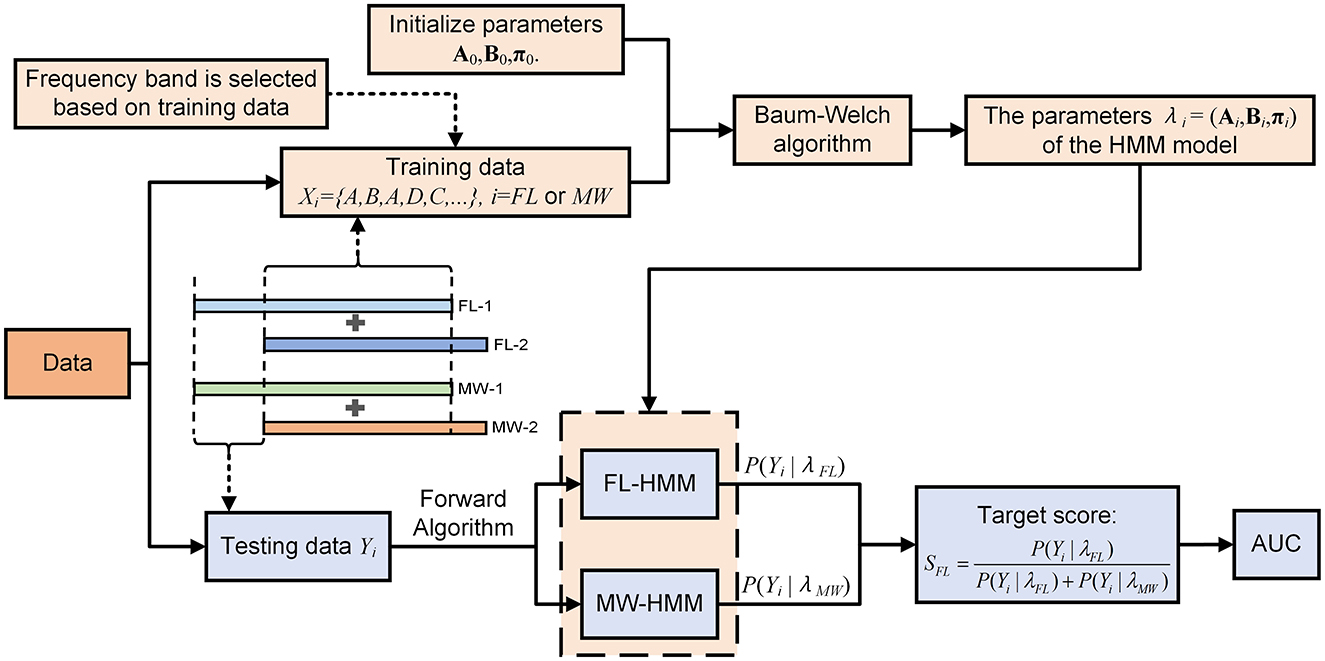
Figure 3. Flowchart of our method for detection of mind-wandering via HMM.

3 Results 3.1 Static analysis results

First, we conducted statistical analysis on a multilayer network created from EEG data from all trials (of the same condition) of all 14 participants. Since one network was made from the data in the entire trial, this is a static analysis. We examined the edges, nodes, and inter-layer heterogeneity under mind-wandering or focused learning.

We found significant differences in intra-layer connections within the multilayer network across frequency bands (Figure 4A). In the AEC layer, significant differences (indicated by triangles) were observed in the edges F3-O1 and F4-T3 across the four frequency bands. Significant differences in edges were mainly concentrated in the delta, alpha, and beta frequency bands. In the IPLV layer, significant differences in edges were mainly concentrated in the theta band.

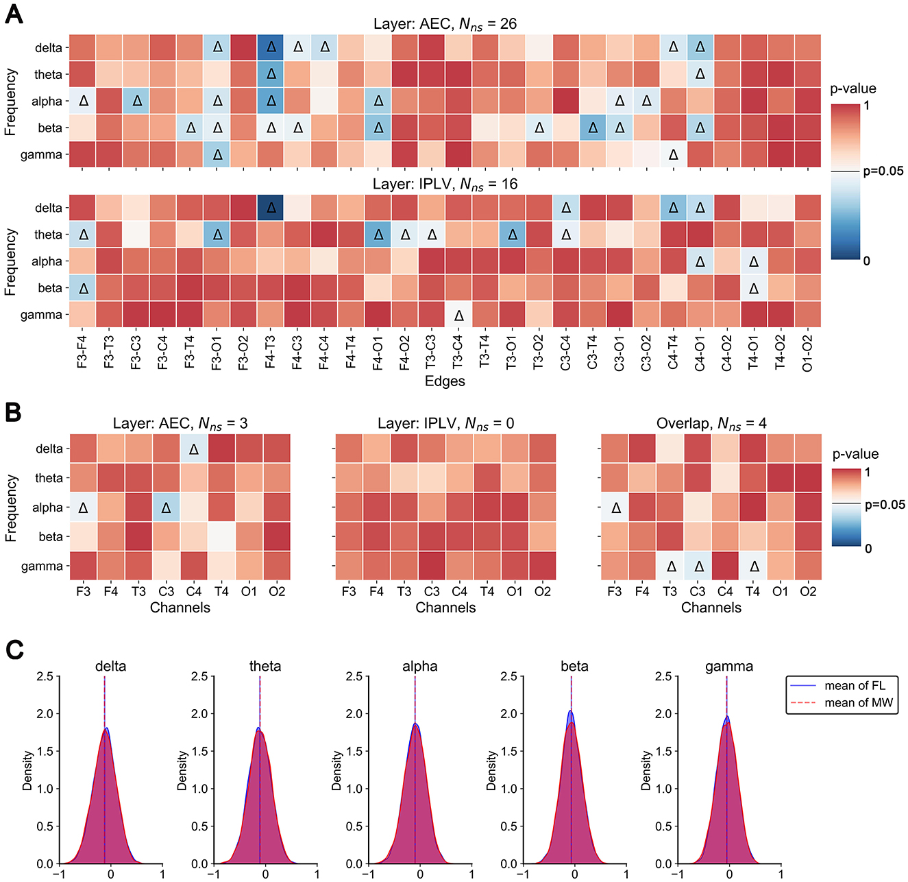
Figure 4. Static analysis results. (A) P-value plot of significant differences in edge weights between MW and FL. Color in the heat map indicates the p-value of the statistical test. Triangles indicate significant differences. (B) P-value plot of significant differences in node closeness centrality between MW and FL. (C) Histograms (across participants and trials) of Pearson correlation values between corresponding edges of the two layers.

We found three significant differences in the node closeness centrality (single layer) of the AEC layer in the delta and alpha bands (Figure 4B). However, we found no significant difference in the node closeness centrality in the IPLV layer. We found four significant differences in the overlapping node closeness centrality (entire multilayer network) in the alpha and gamma frequency bands.

Finally, we examined inter-layer heterogeneity via Pearson correlation of intra-layer connections (for each participant). This distribution of correlation coefficients (among participants and trials) is presented in Figure 4C. The analysis results indicate that the majority of inter-layer correlation coefficients are relatively low, predominantly concentrated around 0. This means there was not much in common in the structure between the layers.

3.2 Dynamic analysis results

We examined differences in the dynamic features computed from the multilayer network state sequences during FL vs. MW, pooling data across participants-trials (Figures 5, 6).

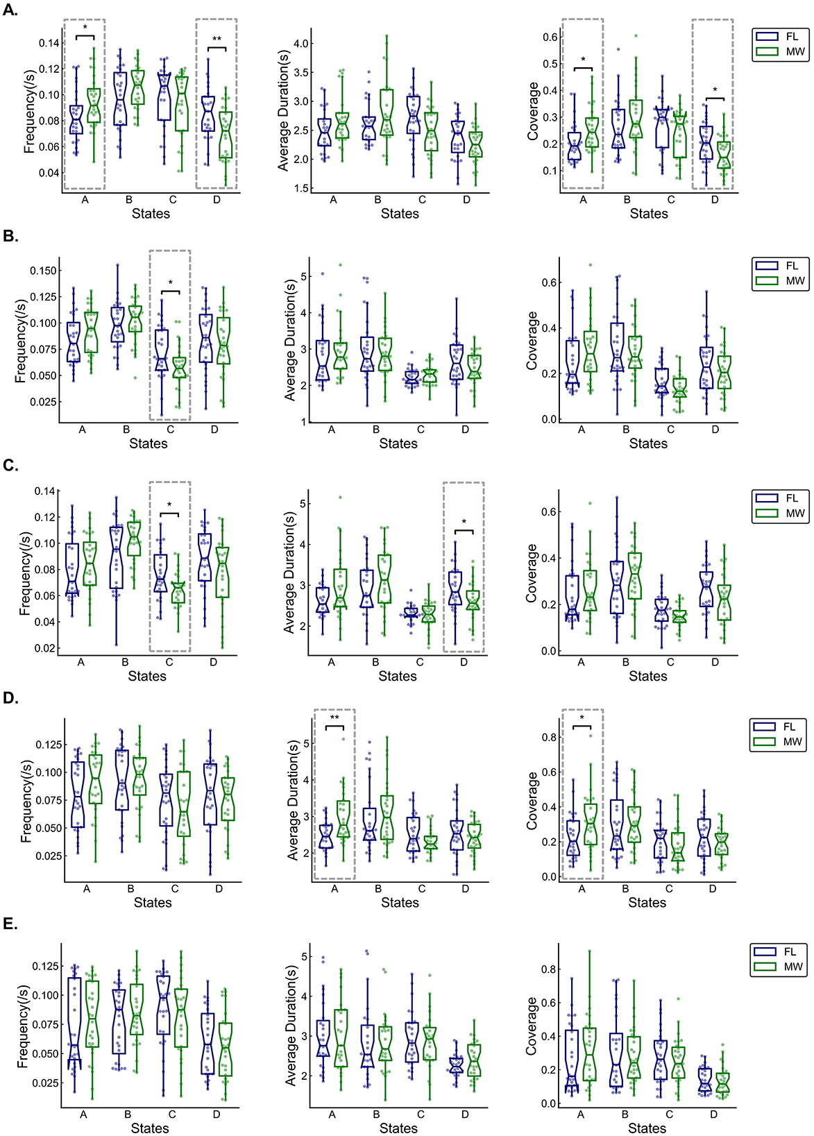
Figure 5. Box and whisker plots (across participants) of occurrence frequency, average duration, and coverage of each multilayer network state for delta (A), theta (B), alpha (C), beta (D), and gamma (E) frequency bands. Statistical significance (dashed boxes) was set at 0.05. *p < 0.05, **p < 0.01, ***p < 0.001.

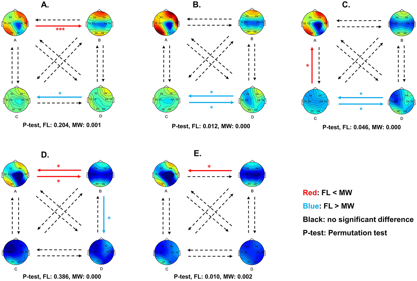
Figure 6. Diagram of multilayer network state transition probability differences between MW and FL for delta (A), theta (B), alpha (C), beta (D), and gamma (E) frequency bands. Red arrows indicate a significantly higher transition probability in MW compared to FL, while blue arrows indicate a significantly lower transition probability. Statistical significance was set at 0.05. *p < 0.05, **p < 0.01, ***p < 0.001.

For the delta frequency band (Figure 5A), MW had a significantly higher occurrence frequency (p = 0.042) for the multilayer network state A. MW had significantly lower the state D frequency (p = 0.009), state A coverage (p = 0.028), and state D coverage (p = 0.024). As shown in Figure 6A, the transition probability from state A to state B was significantly higher for FL (p = 0.000). The transition probability from state D to state C was significantly lower for FL (p = 0.011). The permutation test checking for fully random transitions yielded p=0.204 for FL and p = 0.001 for