To predict individual patient time courses we employ and compare different types of feed-forward or recurrent neural networks (RNNs). Architectures are optimized to cope with the relative sparsity of clinical data. As an alternative, we consider a simple semi-mechanistic model having a limited number of parameters which can be estimated based on individual patient data. We also employ and compare different learning methods for the neural network models including transfer learning from the semi-mechanistic model to allow training of individual networks. We explain these approaches in the following. A more comprehensive presentation is provided in the supplement, Section 1.1 (Online Resource 1). To compare the approaches, we consider real patient data as explained in the following section.

Patient data

We consider patient data from the NHL-B study comparing CHOP-like therapies of high-grade non-Hodgkin’s lymphoma in young and elderly patients (Wunderlich et al. 2003; Pfreundschuh 2004a, b). Patients received either 6xCHOP-14/21 or 6xCHOEP-14/21. Relatively dense data of blood counts are available for most of the patients. Since we aim at predicting individual next cycle platelet toxicity, we here consider patients with platelet data available for at least four therapy cycles and more than one blood count in the first cycle. We exclude patients who received platelet transfusions. This results in a total of 360 patients eligible for analysis.

To assess the impact of data sparsity on prediction performance, patients are stratified into two groups. The first group comprises 135 patients for which at least five platelet counts are available per cycle. This group represents patients whose individual platelet dynamics is well-covered by the available data. All other selected patients are summarized in the second group, representing reduced coverage of the platelet dynamics. Due to often strongly fluctuating dynamics and deeper nadirs, we expect less favorable prediction performances for the 14 day CHO(E)P therapies (d14) compared to the 21 day (d21) schedules. This also has been observed by Kheifetz and Scholz (2019). Thus, we consider four groups in the following analyses, denoted by De14/De21 for patients with dense measurements and Sp14/Sp21 for patients with sparse coverage of their individual platelet dynamics.

Semi-mechanistic model of platelet dynamics

As a reference to our NARX modeling, we consider a semi-mechanistic model of platelet dynamics under chemotherapy proposed by Friberg et al. (2002). This is a simple compartment model describing proliferating stem cells maturing into circulating blood cells. Maturation is modeled by three sub-compartments with first order transitions with transit time MTT. The feedback strength of the circulating compartment towards the proliferating compartment is represented by parameter \(\gamma\). Individual steady-states can be defined by parameter \(C_0\).

The treatment effect of chemotherapy is modeled by a step-wise toxicity function acting on the proliferation compartment. We assume a simple step-function returning to zero after one day. The step height represents the dose of the chemotherapy normalized to the body surface area. The individual toxic effect is represented by parameter \(E_\) multiplied to this dose level. Model equations and parameter ranges are presented in the supplement, Section 1.2 (Online Resource 1). Individual parameters can be derived based on likelihood optimization of the agreement of model and data penalizing strong deviations from the population average. Details are explained in the supplement, Section 1.2 (Online Resource 1).

NARX modeling

Nonlinear auto-regressive models with exogenous inputs (NARX) are a class of models suitable to describe dynamics of discrete time series data affected by external factors. Dynamics are captured by learning a functional relationship between observations or predictions at previous time steps, an externally imposed input function, which in our situation is the applied therapy, and the current state. In our situation, this function is learned via neural networks, further called NARX neural networks. All NARX neural networks are recurrent neural networks (RNNs), and the recurrent connection between the output of the network and the input is formed by a so-called tapped delay line (Siegelmann et al. 1997). In this work, we compare different network architectures regarding their learning abilities and prediction performances.

To assess and improve prediction performances, we consider different architectures of the NARX modeling framework. First, we consider a simple feed-forward network for coupling as proposed by Steinacker et al. (2023). We call this architecture ARX-FNN in the following. In such a network, information only flows in one direction through the network, from the input nodes through potential so-called hidden layers of nodes to the output nodes of the network. We compare this simple framework with more complex alternatives. Specifically, we consider a so called gated-recurrent unit (GRU) network (Cho et al. 2014), which replaces the FNN by an RNN (ARX-GRU). In addition to the FNN weights, RNNs have hidden states which store the past contextual information of an input sequence. This architecture allows the network to memorize relevant information for a longer period of time or neglect such information if not required to improve prediction. Details on the chosen network architectures are given in the supplement, Section 1.1 (Online Resource 1).

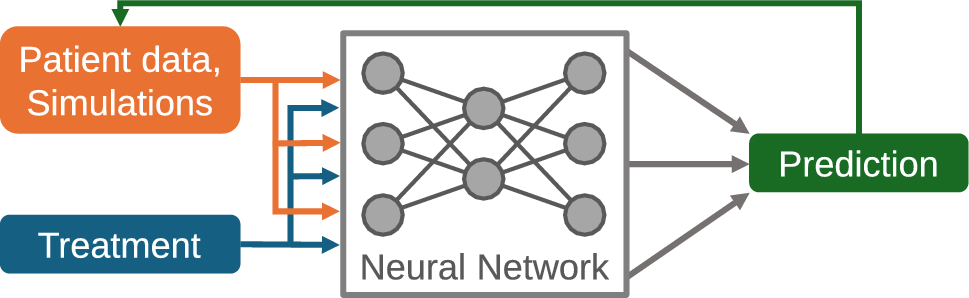
Prediction approach using NARX models

We aim at predicting individual time courses of platelet dynamics. The exogenous input represents applications of cytotoxic drugs. Essentially, the network predicts daily platelet counts based on measured or predicted values at previous days considering the therapy input. In detail, the input of the individual network is a vector of the present and, depending on the architecture, past predicted or observed daily platelet counts, and, as exogenous input, the chemotherapy drug concentration. Since patients are untreated at study inclusion, we assume that platelet histories of patients are in steady-states equal to the respective baseline measurements of patients. We utilize this assumption to start the prediction process. The output of the networks is the platelet count predicted for the next day. Through iteration, the prediction of complete individual time courses is obtained. Details on the different architectures can be found in the supplement, sections 1.1 and 1.4 (Online Resource 1). Figure 1 illustrates our modeling concept.

Fig. 1

NARX neural network models for the purpose of predicting individual platelet dynamics under chemotherapy. The neural network is used to predict future platelet counts of a patient based on previous measured or predicted counts and the provided therapy. The architecture of the neural network can be modified and learned based on individual time series data of patients under treatment

For predicting individual patient dynamics with our NARX frameworks, it is necessary to scale and transform the patient data. First, we log-transform platelet counts due to their log-normal shape of distribution. We further scale the data such that the log-transformed range between degree four thrombocytopenia, \(\times 10^\hbox \) and the average initial state in the Sp group, \(\times 10^\hbox \) (see below), corresponds to the range \([-0.5, 0.5]\) for ARX-GRU models, and \([-1, 1.5]\) for ARX-FNN models. These ranges are the result of a hyperparameter optimization step. Details are provided in the supplement, Section 1.4 (Online Resource 1). Of note, this scaling does not affect the comparability of the fitness measures between models, as scaling is not applied when calculation these measures.

Transfer learning approach for neural network models

Transfer learning (TL) techniques are developed to cope with sparse data problems in machine-learning (Pan and Yang 2010). We here adopt a transfer from (semi-)mechanistic models as proposed recently by us and others, e.g. Steinacker et al. (2023); Kleissl et al. (2023); Zabbarov et al. (2024). In more detail, we parameterize the semi-mechanistic model for given individual patient data and simulate dynamics for different therapy scenarios including the actually given therapy schedule (Steinacker et al. 2023). Details can be found in the supplement, Section 1.3 (Online Resource 1). These simulated dynamics were used to pre-train our neural network for the respective individual patient. The semi-mechanistic model is learned on the same data as the neural network models.

After pre-training, the weights of model inputs and hidden layers remained unchanged. Only weights of the linear output function are re-calibrated based on patient’s real data. This step ensures that learned dynamics from the semi-mechanistic model are preserved while transferring the model to the real patient dynamics. Finally, a fine-tuning step is employed, re-training the whole model with the patient’s real data with a lower learning rate. The adaptation of the linear output and the final fine-tuning are carried out consecutively. Details on regularization during the transfer learning procedure and the fine-tuning can be found in the supplement, Section 1.3 (Online Resource 1). Values of hyperparameters, such as learning rates during the training process, can be found in the supplement, Section 1.4 (Online Resource 1), as well as the provided code repository. To assess the impact of pre-training on prediction performances, we compared this approach with a standard approach without pre-training. Scenarios are denoted "with TL" respectively "without TL" in the following. We provide a visual summary of the learning approaches as a flowchart in the supplement, Section 1.5 (Online Resource 1).

Methods to reduce overfitting

Over-parametrization is a well-known problem of neural network models. We employ multiple methods to reduce overfitting during training of the individual networks. Depending on network architecture and training strategy, we combine different standard methods as explained in the following. Details of the specific methods are given in the supplement, Section 1.3 (Online Resource 1).

Methods acting on the network structure comprised pruning and weight regularization. Pruning describes the removal of nodes or weights from the network to reduce the number of free parameters and to improve generalization performance (LeCun et al. 1990). We employ pruning for all training processes considered. The dropout method is a form of non-permanent pruning, where weights are randomly removed from a network with a specified frequency (Srivastava et al. 2014). We apply this method only for training modes without TL. Weight regularization adds a penalty to the objective function of the model, which consists of the squared sum of the network weights. It is also known as weight decay (Krogh and Hertz 1991). Again, this technique is applied for all training process.

Still, neural networks suffer from over-parametrization as they tend to assume noisy dynamics in case of larger time distances between measurements. To avoid this behavior, it is necessary to regularize such noisy dynamics. We adopt here exponential smoothing (Brown 1956; Brown and Meyer 1961; Holt 2004), which acts as a low-pass noise filter. We apply this method to the network output in the following way:

$$\begin }'_0&= }_0, \end$$

(1)

$$\begin }'_i&= \alpha }_i + (1-\alpha )}'_, \end$$

(2)

with smoothing factor \(\alpha \in [0,1]\), implemented as a trainable parameter of each individual neural network model. Here, the model prediction at day i corresponds to \(}_i'\) while the regressed variable \(}_i\) is used in the auto-regressive feedback loop of the network. To encourage the network to employ exponential smoothing, we include a respective smoothness penalty term in the objective function. The complete formula of the objective function is provided in the supplement, Section 1.3 (Online Resource 1). We also provide the average learned smoothing factor \(\alpha\) per patient group, network architecture and learning approach in the supplement, Section 1.4 (Online Resource 1).

Another established method to avoid overfitting due to small data-sets is the addition of a noise term to the training data, which can be seen as a form of data augmentation (Goodfellow et al. 2016). It encourages the neural network output to be a smooth function of its input and weights, respectively (An 1996). We add here a Gaussian noise to the scaled network inputs. This augmentation is only active in the training phase, where dynamics of real patient data are learned.

Comparison of prediction performances

We use two fitness measures to assess and compare prediction performances between our learning frameworks. First, we consider the modified mean-squared error (SMSE), which is also employed during network training on real patient data. Since time points of measurements are not exactly known, we use a weighted average of the mean squared error over three days (weight 0.3 for the previous or next day, weight 1.0 for the actual day). This performance measure is useful for training individual models and comparing them in terms of accuracy of platelet predictions. The formula to calculate the SMSE reads as follows,

$$\begin = \frac \left[ \sum _i (y_i - }_i)^2 + 0.3 s \left( \sum _i \left( (y_i - }_)^2 + (y_i - }_)^2\right) \right) \right] , \end$$

(3)

where \(y_i\) denotes the observed and \(}_i\) the predicted log-transformed cell count at day i, and N denotes the total number of observations used for evaluation. Log-transformed cell counts emphasize the nadir phase of the cell dynamics, which is clinically relevant. Model scaling as mentioned in Sect. 2.4 was not applied for the purpose of SMSE calculation. Thus, models are comparable regarding SMSE. This measure is also used in the objective function during learning. The complete form of the objective function and all model hyperparameters are provided in the supplement, Section 1.3 and 1.4, respectively (Online Resource 1).

For a clinically more useful and interpretable measure of prediction performance, we determine the difference of predicted and observed thrombocytopenia degrees (\(DD_\)) at the nadir phase of each therapy cycle. To determine the thrombocytopenia degree, we adhere to the criteria of the National Cancer Institute (National Cancer Institute 2009). The degree is classified as follows for cell count C:

$$\begin \text = 0,\quad C> \times 10^\hbox ,\\ 1,\quad C> \times 10^\hbox \text C \le \times 10^\hbox , \\ 2,\quad C> \times 10^\hbox \text C \le \times 10^\hbox ,\\ 3,\quad C > \times 10^\hbox \text C \le \times 10^\hbox ,\\ 4,\quad C \le \times 10^\hbox . \end\right. } \end$$

(4)

The \(DD_\) is calculated as follows,

$$\begin DD_ = \frac | d_ - }_ |}, \end$$

(5)

where c denotes the number of calibration cycles utilized, t denotes the cycle for which the prediction is made, \(P_t\) is the set of patients with measurements for that cycle, d denotes the observed thrombocytopenia degree in that cycle for patient p, and \(}\) is the respective prediction at this time point. This fitness measure was proposed by Kheifetz and Scholz (2021) to evaluate and compare predictive performances between models. The advantage of this fitness measure is that it determines clinically relevant differences between predicted and observed platelet counts in terms of toxicity grades.