This study is a retrospective study conducted on patients diagnosed with complete TGA who underwent ASO at Seoul National University Children’s Hospital from January 1, 2003, to December 31, 2013. Our analysis involves cardiac computed tomography (CT) images of patients who received cardiac CT scans between the ages of 8 and 18 within this patient cohort. The selected age range of 8 to 18 years ensures the inclusion of long-term follow-up data, as neo-aortic root dilatation is primarily a long term complication post-ASO [3, 4]. Additionally, we included patients aged 8 years and older because they are more likely to have a body weight of at least 30 kg and a body surface area (BSA) of at least 1.2 m2, approximating adult body size. The upper limit of 18 years is based on the reference population used by Lopez et al. for Z-score calculations [17]. The patient groups are categorized into three groups: severe aortic dilation (Z-score ≥ 4) (Group A), mild aortic dilation (2 < Z-score < 4)(Group B), and a healthy control group (Z-score \(\le 2)\)(Group C) consisting of adolescents aged between 8 and 18 who underwent cardiac CT scans due to chest pain but exhibited no structural or functional abnormalities. Following the age-matching process, the complete cohort consisted of fifteen patients, divided into three groups: 5 individuals in Group A, 5 in Group B, and 5 in Group C. This study excluded patients who underwent ASO after the diagnosis of TGA and subsequently deceased during the study period, as well as those with combined arch anomalies requiring staged operations. This study was approved by the Institutional Review Board of the Seoul National University Hospital (IRB number: H-2311–002-1481).

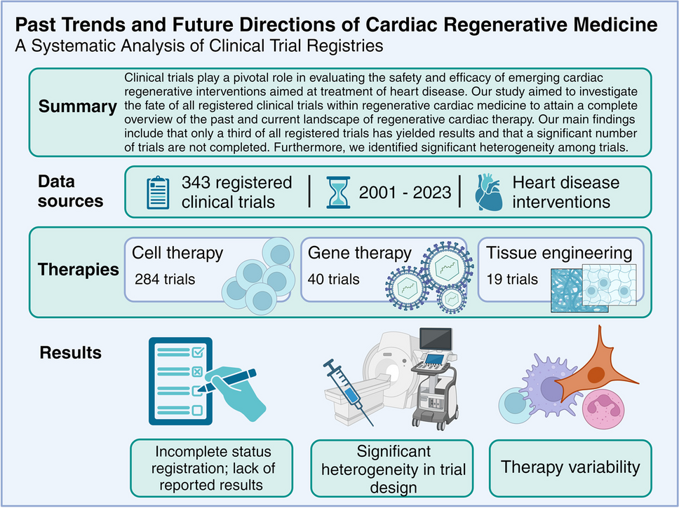
Retrospective measurements were conducted on images obtained from cardiac CT. Neo-aortic diameters were assessed at four specific levels: 1) neo-aortic valve annulus, from hinge point to hinge point; 2) neo-aortic sinus of Valsalva, from the internal edge to the internal edge; 3) neo-aortic sino-tubular junction (STJ) by internal edge to internal edge; and 4) mid-ascending aorta, at the level of the mid main pulmonary artery, from hinge point to hinge point. For precise selection of the accurate hinge point and level, we simultaneously utilized axial, coronal, and sagittal views in two-dimensional images (as shown in Fig. 1) as well as three-dimensional reconstructed images (as shown in Fig. 2). By combining these 2D image cuts and 3D reconstruction images, we ensured accurate measurement of the diameters. For the measurement of the diameter at the mid-ascending aorta level, we recorded both the minimum and maximum diameters and then calculated the average diameter. To account for the range in body size for neo-aortic measurements during 8–18 years, Z-scores for each patient were calculated using the pediatric reference recommended by Lopez et al. [17], which covers the age range from 0 to 18 years. The body surface area (BSA) was calculated using the Haycock method [18]. Severe dilation was defined as a Z-score of ≥ 4 in any component of the aortic root, encompassing the aortic valve annulus, sinus of Valsalva, sino-tubular junction, or ascending aorta. Mild dilatation was characterized by a Z-score between 2 and 4 in any of the aforementioned components of the aortic root.

Measurement of the diameter of the neo-aortic valve at the annulus level. For the precise selection of the accurate hinge point and level, axial (A), sagittal (B), and coronal (C) views in two-dimensional images were simultaneously utilized

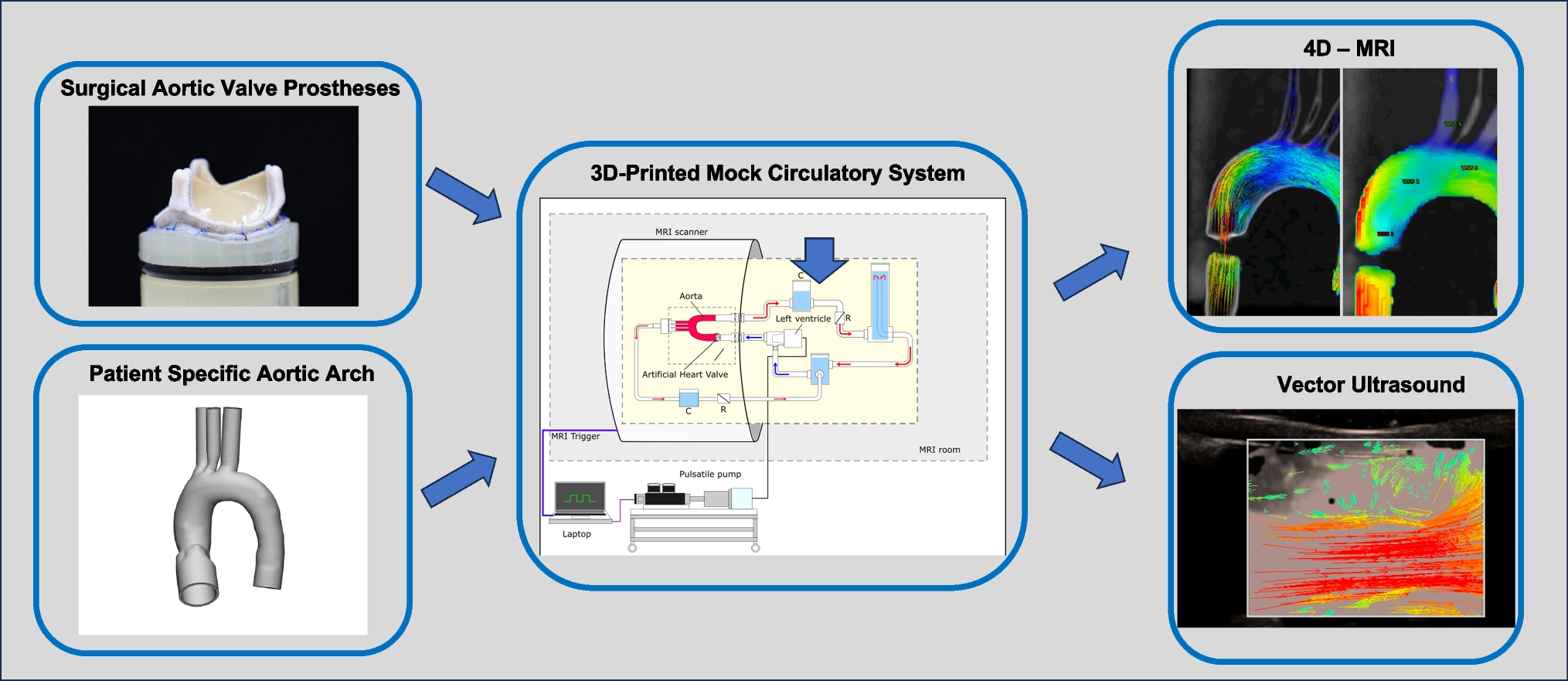
Measurement of wall shear stress, vorticity, and aortic arch angle. A Two-Dimensional Slices at Different Aortic Locations. Two-dimensional slices were obtained perpendicular to the centerline of the aorta model at five locations. Plane 0 (Aortic Root): Positioned one diameter away from the two-dimensional slice above the annulus. Plane 1 (Proximal Ascending Aorta): Located by moving one diameter in the inlet direction from the second cross-section. Plane 2 (Distal Ascending Aorta): Positioned just before the first bifurcation. Plane 3 (Aortic Arch): Placed just after the last bifurcation. Plane 4 (Descending Aorta): Defined by moving two diameters in the descending aorta direction from the third cross-section. Vorticities were calculated over these two-dimensional slices at each of the five different locations along the centerline. B Wall Shear Stress Calculation. Wall shear stresses were time-averaged over one cardiac cycle and area-averaged over the region of interest, as indicated in Fig. 2B. The region extended proximally from the STJ to a distance of one diameter for calculating the WSS in the aortic root (sky blue color). Using the planes labeled as Plane 1–4 in Fig. 2A as references, a region above and below each plane within a distance of 0.5 diameter was defined. In this space, WSS measurements were taken for the proximal ascending aorta (red), distal ascending aorta (yellow), aortic arch (green), and descending aorta (blue). C Measurement of the aortic arch angle involved identifying the highest point of the centerline of the aorta (Point A) and drawing a tangent line from this point. The second line was created by moving one diameter parallel to the tangent line and determining two points where the centerline intersected with this line (Point B and C). The angle was subsequently calculated between line AB and line AC. WSS: Wall shear stress

The factors influencing aortic root dilatation in patients with TGA who underwent ASO were chosen based on literature reviews and include male sex, the presence of VSD, Taussig-Bing anomaly, arch anomalies such as interrupted aortic arch or coarctation of the aorta, bicuspid neo-aortic valve, coronary artery abnormality, pulmonary artery banding before ASO, great artery size discrepancy, coronary transfer technique, neo-aortic regurgitation within 1 year after ASO, and arch angle [5,6,7,8,9,10,11,12]. In the study, due to missing preoperative size data, "great artery size discrepancy" was verified from surgical records or echocardiograms, where the pulmonary artery exceeded 1.5 times the aorta size.

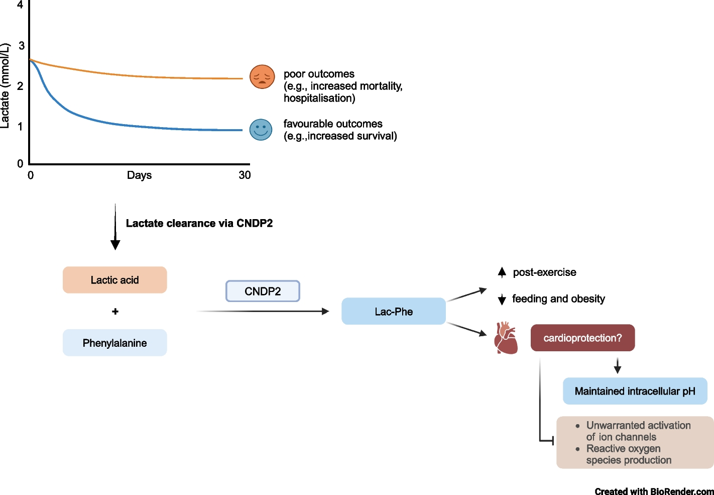
We used cardiac CT images of TGA patients who underwent ASO, including those with severe neo-aortic root dilatation, mild neo-aortic root dilatation, as well as images from a healthy control group. The SimVascular software, an open-source tool [19], was utilized for the segmentation of aorta, construction of anatomical models, and the simulation of blood flow. The modeling and simulation steps encompassed geometry acquisition, description of boundary conditions, selection of computation type and parameters, simulation, and post-processing (e.g. visualizations) of numerical data. Initially, three-dimensional paths were generated by manually tracking the lumens of the aorta visible in the CTA images. Subsequently, the vessel underwent segmentation, determining its contour at central points. At each cross-section along the centerline, we determined which parts of the medical image depicted the object of interest, which was achieved through the level set method and threshold setting. These two-dimensional lumen segmentations were then lofted into a three-dimensional model, representing the anatomical model of aorta.

For the simulation of blood flow, we employed svSolver, integrated with SimVascular. This solver utilizes a stabilized finite element method with linear tetrahedral elements. The governing equations used to simulate blood flow were the incompressible Navier–Stokes equations and the continuity equation. Finite element meshes were generated using the TetGen package, an open-source tool [20], facilitated by SimVascular. The vessel wall was assumed to be rigid. The simulations produced time-resolved fields of blood velocity and pressure throughout the aorta model. In all simulations, blood was assumed to be a Newtonian fluid, with a viscosity of 0.04 dynes/cm2 and a density of 1.06 g/cm3. The non-Newtonian effects of blood, typically observed in vessels with diameters smaller than 300 μm, were not taken into consideration in this study [21]. We acknowledge that the non-Newtonian fluid model (e.g. Carreau-Yasuda model) can improve the simulation realism, however, given the smallest lumen diameters analyzed were on the order of 1 mm, we assume that the Newtonian fluid model can accurately predict the flow behaviors in the aorta where the shear rate is expected to remain above ~ 100/s. In this shear rate regime, the dynamic viscosity is largely unchanged [22, 23].

At the inlet of the aorta model (plane above the annulus), we prescribed a time-resolved aortic waveform obtained from healthy patients scaled to match the estimated cardiac output of each patient using their age and BSA [24]. Estimated cardiac output ranges 3.8 to 6 L/min depending on the patient. The Reynolds number associated in our simulation based on the cardiac output and the vessel diameter, \(Re=\frac\) ranges between 1008– 1671, with mean ± standard deviation as 1333 ± 210. In this regime, the flow can be assumed as laminar or transitional flow.

Boundary conditions for blood flow at the outlets of the aorta, brachiocephalic arteries, and carotid arteries were imposed using an open-loop lumped parameter network model. The lumped parameter model was used to simulate the physiological hemodynamic response of downstream vessels in a volume-averaged manner and was prescribed as a boundary condition. This network employs an electrical circuit representation to model blood flow commonly referred to as 3-element Windkessel model consisting of two resistances and capacitance of distal vasculature [25]. These parameters underwent tuning to ensure that the simulations accurately reflected patient-specific clinically measured aortic pressure. Specifically, we iterate simulations with initial guess of the resistances and capacitances until it converges to the patient’s maximum and minimum pressure. The difference between the simulated and measured blood pressures in patients was 5.1% ± 3.4%. The distribution of flow among carotid arteries was determined based on the modified Murray’s law with an exponent of 2.0 [26].

For all 15 patients, a time step size of 0.001 s was used. We checked the time step convergence by decreasing the time step to 0.0005 s, which is half of the implemented time step, and verified that all the presented results were unchanged within 3% errors. At least eight cardiac cycles were simulated and the only last 1 heart cycle data were used to eliminate the initial transient effects. The number of total time steps varies between 8000 and 15000 depending on the patient. The number of time steps was determined by performing simulations until the blood pressure and other hemodynamic values converged within 1% of variabilities compared to the previous cycle for each patient.

We used high-resolution meshes to resolve detailed blood flow patterns. We applied an edge size of 0.8 mm for all patient models after conducting a mesh independence study, by subsequently increasing the number of mesh up to 8 million elements and confirming an appropriate edge size for mesh independence compared to the highest-resolution mesh. In addition, boundary layer meshing technique, which places smaller size meshes near the vessel wall, was added to accurately capture the wall shear stress. With these strategies, we achieved mesh convergence for both wall shear stress and vorticities within 10% errors compared to a refined mesh with double-sized elements. The number of elements ranges from 1.8 million to 5.1 million, averaging 3.5 million elements. The number of boundary layer meshes is 3, the layer decreasing ratio is 0.8, and the portion of edge size is 0.5 mm.

We note that the svSolver was extensively validated against in-vivo, in-vitro measurements, and intra-CFD group benchmark tests [27,28,29]. Previous validations studies showed excellent consistencies between aortic flow fields measured by svSolver and those by 4-D magnetic resonance imaging techniques [30, 31]. We believe that application of svSolver is suitable and provides credible quantitative visualization results of aortic flows.

After the simulations, we conducted post-processing on the hemodynamic variables. Two-dimensional slices perpendicular to the centerline of the aorta model were obtained at five specific locations (Fig. 2A). The first slice (Plane 0) was measured at the proximal site one diameter distanced from the two-dimensional slice above the annulus. The second slice (Plane 1) was measured at the proximal site one diameter distanced from the brachiocephalic artery. The third slice (Plane 2) was measured just before the brachiocephalic artery. The fourth slice (Plane 3) was measured right next to the left subclavian artery. The fifth slice (Plane 4) was measured at a location two diameters distanced from Plane 3.

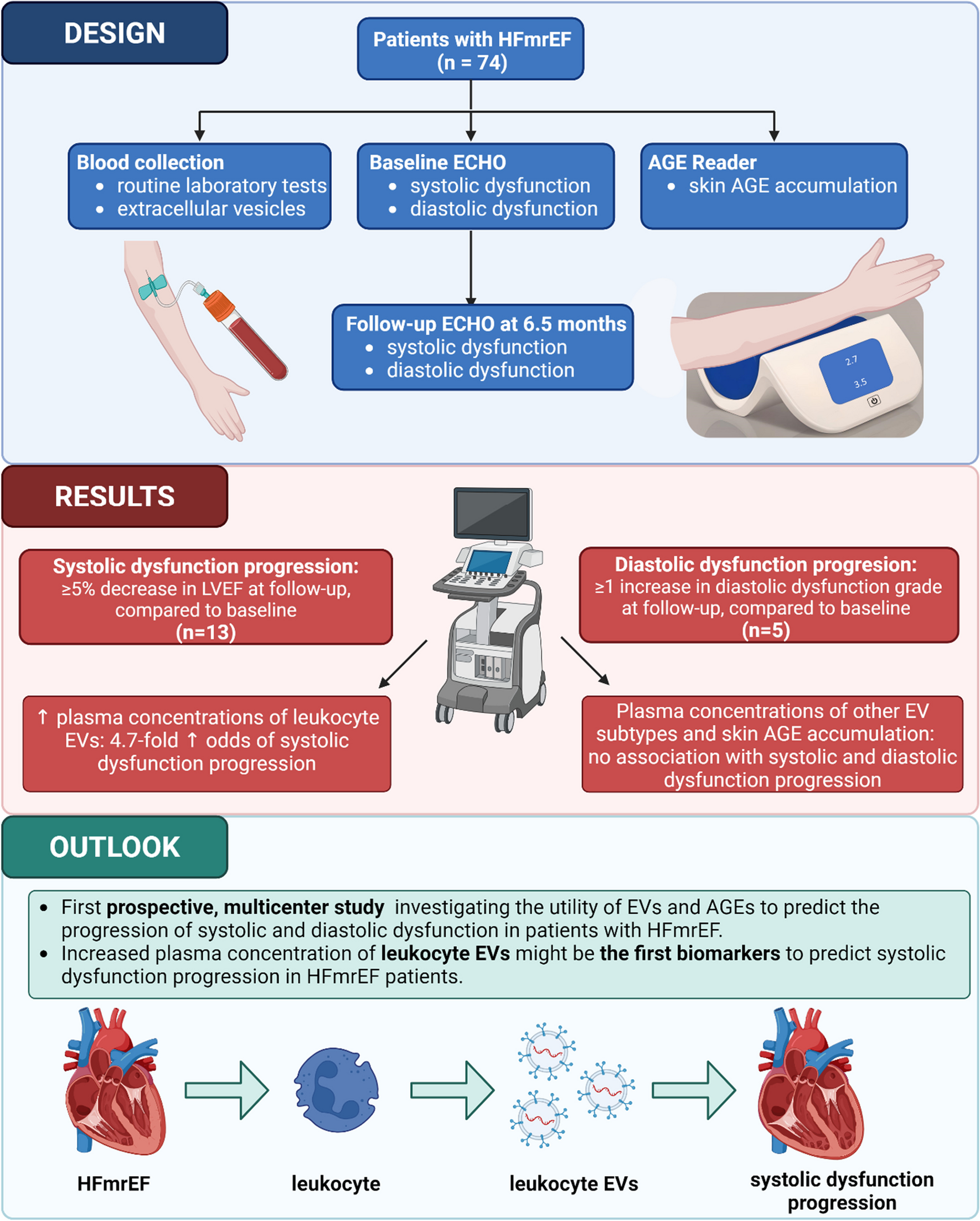
In this study, we post-processed the CFD data and quantified hemodynamic metrics of clinical interest to characterize the hemodynamic differences among patient groups. Time-averaged wall shear stress (TAWSS) is one of the key hemodynamic parameters associated with many cardiovascular diseases thus being used for advanced treatment of cardiovascular disease. Low TAWSS is known to be associated with endothelial cell dysfunction, arterial plaque progression [32], vein graft failure, pulmonary hypertension [33], and aneurysm growth [34, 35]. Also, we investigated vorticity to study the dynamic characteristics of aortic flow in response to changes in the aortic root. Vorticity quantitatively measures how ‘swirly’ blood flows and we hypothesized that a straight blood flow pattern is more favorable than recirculating flows.

Wall shear stresses were time-averaged over one cardiac cycle, and area-averaged over the interested region near the sinus and the slice boundaries (Fig. 2B). We defined a region extending proximally from the STJ to a distance of one diameter to calculate the WSS in the aortic root (represented by the sky-blue color). Additionally, using the planes denoted as Plane 1–4 in Fig. 2A as references, we defined a region above and below each plane within a distance of 0.5 diameter. In this space, we measured the WSS for the proximal ascending aorta (red), distal ascending aorta (yellow), aortic arch (green), and descending aorta (blue).

The aortic arch angle was measured by first identifying the highest point of the centerline of the aorta (Point A) and drawing a tangent line from this point. Subsequently, a second line was created by moving one diameter parallel to the tangent line and determining two points where the centerline intersected with this line (Point B and C). The angle was then calculated between line AB and line AC (Fig. 2C).

Vorticities were calculated by taking spatial derivatives of the velocity components. Vorticity magnitudes were averaged over the two-dimensional slices and then averaged over the cardiac cycle at each five different locations along the centerline (Fig. 2A).

All data analyses were performed using SPSS statistics 25.0 (IBM, Armonk, NY, USA) and GraphPad Prism software. Data is presented as median and ranges. Not normally distributed data was compared between groups using the Mann–Whitney test, Fisher’s exact test and Kruskal–Wallis test. T-test was employed for normally distributed continuous variables between two groups. As appropriate, p < 0.05 was considered significant.