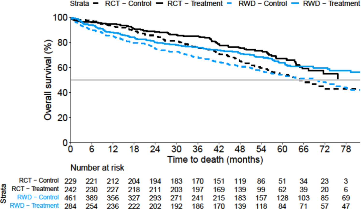
Figure 1 displays unweighted (unadjusted) survival curves for the four cohorts, and Fig. 2 shows the ATE-adjusted Kaplan–Meier curves. The RCT results were recalculated without stratification, as stratification data were not available in the EC. This resulted in a revised RCT HR = 0.69, 95% CI 0.51, 0.93 with a two-sided p value of 0.014 (Table 1), as compared to the original RCT result of HR = 0.71 and the multivariable adjusted RCT estimate of HR = 0.74. Table 1 shows a comparison of point estimates between the EC and RCT results (ATE HR = 0.76, ATT HR = 0.84 and ATO HR = 0.87). The PH assumption was doubtful to be met with p = 0.002, p = 0.035 and p = 0.064 for ATE, ATT and ATO (Table 1). The RCT RMST treatment difference was 5.6 months (p = 0.025, two-sided), compared with 5.9 months for the EC using the ATE (p = 0.016). As for the HR, the ATO-weighted and ATT-weighted RMST results were again closer to the null hypothesis (3.2 and 3.4 months treatment difference, respectively) when comparing with the ATE (Table 1).

Unweighted overall survival by cohort, Kaplan–Meier curves for the multiple myeloma case study. RCT randomised controlled trial, RWD real-world data

Average treatment effect (ATE)-weighted overall survival comparing the randomised controlled trial (RCT) treatment arm with the real-world data (RWD) comparator cohort, Kaplan–Meier curves for the multiple myeloma case study

See Table 9 in the ESM for the distribution of demographic and baseline characteristics. When checking the covariate balance, the standardised mean differences were observed to be < 0.11, indicating an improved balance of measured covariates across treatment groups after applying PS weights (Table 10 in the ESM). Note that balance in unmeasured covariates cannot be assessed. Propensity score and weight distributions are displayed in Fig. 3 and Table 11 in the ESM.

Table 12 in the ESM shows ATE results applying a model without MI, and a MI model including only covariates with missingness < 35%. These results were similar to the original ATE analysis results.

Interestingly, the PH assumption appeared reasonable within both data sources (within the RCT and within the RW data) but seemed to be compromised when using one arm from the RCT and a comparator cohort from the RW data (Figs. 1 and 2), showing the potential for the non-robustness of the PH assumption when mixing two data sources in the EC setting. Figure 4 in the ESM shows an ATE comparison of the internal control and the EC, where the potential deviation from the PH assumption becomes visible.

Figure 3 displays unweighted (unadjusted) survival curves, and Fig. 4 the ATE-adjusted Kaplan–Meier curves, for which the proportionality of hazards was considered to be a reasonable assumption (Table 2). Table 2 in the ESM displays the association of PS covariates with OS as per the RCT. Table 2 reports ATE, ATT and ATO estimates together with the RCT results. The RCT estimate of HR = 0.64 was seen to be empirically lower than the ATE, ATT and ATO results (HR range 0.81–0.86). Similarly, the RMST RCT difference of 6.5 months was empirically higher than the ATE, ATT and ATO estimates, which ranged from 2.2 to 3.5 months.

Unweighted overall survival by cohort, Kaplan–Meier curves for the metastatic hormone-sensitive prostate cancer case study. The grey line at the 50% mark denotes a reference line for corresponding median overall survival times. RCT randomised controlled trial, RWD real-world data

Average treatment effect (ATE)-weighted overall survival comparing the randomised controlled trial (RCT) treatment arm with the real-world data (RWD) comparator cohort, Kaplan–Meier curves for the metastatic hormone-sensitive prostate cancer case study. The grey line at the 50% mark denotes a reference line for corresponding median overall survival times

See Table 7 in the ESM for the distribution of demographic and baseline clinical characteristics. Most standardised mean differences were observed to be ≤ 0.20, except for ECOG (0.25 for ATE and 0.29 for ATT), indicating a limited balance in measured characteristics across treatment groups after PS weighting (Table 13 in the ESM). Propensity score and weight distributions are displayed in Fig. 5 and Table 14 in the ESM.

For the ATE, different strategies for handling missing data were applied as a sensitivity analysis. These led to similar estimates of HR = 0.84–0.87 (see Table 15 in the ESM) with the PH assumption being reasonable and RMST differences that ranged between 1.6 and 2.5 months.

A direct comparison of the EC with the internal RCT control group showed numerical but nominally non-significant differences after weighting when using the Cox model (HR = 1.30, 95% CI 0.85, 1.99, p = 0.22) and RMST differences (−4.4, 95% CI −9.6, 0.8, p = 0.097), see Fig. 6 and Table 16 in the ESM. Note that the p-value testing the PH assumption for this comparison was p = 0.28 and Kaplan–Meier curves did not yield strong signals for non-proportionality. When applying the alternative index date, the adjusted analysis resulted in HR = 0.88, 95% CI 0.53, 1.44 for ATE, HR = 0.91, 95% CI 0.54, 1.55 for ATT and HR = 0.78, 95% CI 0.54, 1.13 for ATO, respectively (Table 17 in the ESM).

The TTND analyses showed that many RW patients stayed with androgen deprivation therapy alone just for a short time period (in around 20% of patients a subsequent treatment was initiated in the first 3 months), which was different to the RCT. The unweighted HR for TTND was HR = 0.40, 95% CI 0.31, 0.52, as compared to the estimate from the RCT (HR = 0.47, 95% CI 0.41, 0.55 (Table 18 in the ESM). The ATE-weighted analysis resulted in HR = 0.41, 95% CI 0.30, 0.58, and ATT and ATO point estimates were HR = 0.43 and HR = 0.41, respectively. The original RCT RMST difference result was 13.8 months (95% CI 11.1, 16.5) as compared to the ATE, ATT and ATO estimates that ranged from 16.5 to 17.2 months. Corresponding unweighted and weighted TTND figures are available in Figs. 7 and 8 in the ESM.

In Figs. 5a, b 6a, b, 7a, b, the performance metrics bias, type I error and the true coverage proportion of the 95% CI are displayed for the ATE, ATT and ATO, including also the naïve unweighted analysis where no adjustment is applied at all. It should be noted that in the figures the unweighted results do fluctuate slightly for different missingness scenarios because of the nature of performing simulations (using data following a random distribution), though they are constant from a theoretical perspective, as they are independent of any missingness adjustment. 

a Mean bias and 95% confidence interval for the natural logarithm of the hazard ratio [log(HR)] by marginal estimator and factor in case of no unmeasured confounding. The horizontal dashed lines denote a bias of zero. The upper part of the figure is based on the multiple myeloma case study and the lower part of the figure is based on the metastatic hormone-sensitive prostate cancer study. b Mean bias and 95% confidence interval for the natural logarithm of the hazard ratio [log(HR)] by marginal estimator and factor in case of unmeasured confounding. The horizontal dashed lines denote a bias of zero. The upper part of the figure is based on the multiple myeloma case study and the lower part of the figure is based on the metastatic hormone-sensitive prostate cancer study

a Mean type I error and 95% confidence interval for the natural logarithm of the hazard ratio [log(HR)] by marginal estimator and factor in case of no unmeasured confounding. The horizontal dashed lines denote the nominal type I error of 2.5%. The upper part of the figure is based on the multiple myeloma case study and the lower part of the figure is based on the metastatic hormone-sensitive prostate cancer study. b Mean type I error and 95% confidence interval for the natural logarithm of the hazard ratio [log(HR)] by marginal estimator and factor in case of unmeasured confounding. The horizontal dashed lines denote the nominal type I error of 2.5%. The upper part of the figure is based on the multiple myeloma case study and the lower part of the figure is based on the metastatic hormone-sensitive prostate cancer study

a Mean 95% confidence interval coverage percentage and 95% confidence interval for the natural logarithm of the hazard ratio [log(HR)] by marginal estimator and factor in case of no unmeasured confounding. The horizontal dashed lines denote the nominal two-sided coverage of 95%. The upper part of the figure is based on the multiple myeloma case study and the lower part of the figure is based on the metastatic hormone-sensitive prostate cancer study. b Mean 95% confidence interval coverage percentage and 95% confidence interval for the natural logarithm of the hazard ratio [log(HR)] by marginal estimator and factor in the case of unmeasured confounding. The horizontal dashed lines denote the nominal two-sided coverage of 95%. The upper part of the figure is based on the multiple myeloma case study and the lower part of the figure is based on the metastatic hormone-sensitive prostate cancer study

In the figures, the performance metrics bias, type I error and 95% CI coverage are displayed with their 95% CIs for a given factor as the average over all scenarios within the specified factor. As an example, the scenarios with one missing variable are averages over all scenarios where one variable is missing, at 25%, 50% or 75%. As another example, the scenarios with 25% missingness are averages over all scenarios with zero to four missing covariates. The case of no missing data can be looked at in the last panel labelled “Missing Variables” for a zero number of missing variables (Figs. 5a, 6a and 7a).

Ideally, the bias in the simulations would be zero. However, when introducing missing data and unmeasured confounding, some bias was observed (Fig. 5a, b). This bias was observed to be away from the null hypothesis (i.e. in favour of the experimental treatment).

Figure 5a shows that the bias was quite similar for varying HR. Low sample size and trial/comparator ratio may increase the bias especially for the ATT. The larger the missingness and unmeasured confounding, the larger the bias and the more differences between marginal estimators are seen. This is true for both the percentage of missingness within a variable and the number of variables with missing data. Overall, the average bias was lowest for the ATE, followed by the ATO and finally by the ATT.

Scenarios displaying unmeasured confounding (Fig. 5b) did not show any difference between marginal estimators. This is comprehensible because covariates being 100% missing are not associated with any reweighting of MI-derived random values when using within-cohort MI. Numerical estimates show a mean logarithm of the HR bias of around −0.25 for MM and −0.15 for mHSPC (Table 19 in the ESM). For scenarios without any missingness, the bias is approximately zero for all marginal estimators (see also Table 19 in the ESM), as expected.

In the ideal case, the empirical type I error in the simulations would be 2.5% (one-sided), while in the case of unmeasured confounding, a higher average type I error can be expected due to the observed bias in favour of the experimental treatment. Indeed, the average type I error for unmeasured confounding was seen to be 38% for MM and 22–25% for mHSPC (Table 19 in the ESM).

For scenarios without any missingness, the type I error was not significantly different from 2.5%, as expected, and the ATE resulted in estimates that were closest to the nominal alpha of 2.5% (Table 19 in the ESM). For missingness scenarios, the observed type I error differed for the applied marginal estimators. Concretely, the ATE type I error was on average 2.6% and 1.6% for the MM and mHSPC case study simulations, while for ATT this was 14.0% and 4.3%, respectively. The ATO type I error was between the other two marginal estimators by being 8.2% and 2.9% for MM and mHSPC study simulations, respectively (Table 19 in the ESM).

Figure 6a, b show that the type I error increased for increasing sample size and for increasing trial/comparator sample size ratio as expected, as biased analyses in favour of the experimental treatment are known to result in increased type I error rates when the power increases. Figure 6a shows the pattern that the more extreme the missingness, the more differences between marginal estimators: for the simulations based on the MM study, the larger the missingness (for both the percentage of missingness within a variable and the number of variables with missing data), the higher the type I error when applying the ATT and ATO, while the ATE did adhere to the nominal alpha level. For the simulations based on the mHSPC study, the differences were less pronounced, with both ATE and ATO adhering to the nominal alpha level of 2.5%.

Ideally, the true coverage of the 95% CI would be 95%. Indeed, for scenarios with complete data, the true coverage was close to 95% for all marginal estimators, as expected, while for unmeasured confounding scenarios the coverage was estimated to be below 95%. There was no difference between marginal estimators in the case of unmeasured confounding (Fig. 7b), while for missing data scenarios the ATE performed best, ATO performed second best and ATT performed worst (Fig. 7a). Concretely, ATE coverage was 95% for MM and 96% for mHSPC, while ATT coverage was only 82% for MM and 90% for mHSPC (Table 19 in the ESM). The empirical ATO coverage was between ATE and ATT estimates by being 87% for MM and 94% for mHSPC (Table 19 in the ESM).

The observed relative performance patterns were similar for the two case study set-ups, and the observed absolute performance differences were in line with the different number of explanatory covariates, the covariates having different levels of impact and different covariance matrices. A larger bias, type I error and a lower 95% CI coverage was seen in the MM-based simulations compared with the mHSPC-based simulations.

Descriptive statistics for all performance metrics are available in Table 19 in the ESM, together with descriptive p values. Overall, as measured by averages, the ATE performed best (p < 0.001) compared with ATT and ATO regarding all the applied performance characteristics of bias, type I error and 95% CI coverage. Though there was barely any difference within each of the unmeasured confounding scenarios, substantial differences were seen for the missing data scenarios, especially when the missingness was large. However, Table 20 in the ESM displays proportions of how often a specific marginal estimator performed best, and there were a number of scenarios where the ATT and ATO performed best, such that the adequate average performance of the ATE cannot be generalised to all scenarios. As an example, in terms of the performance metric ‘bias’, the ATE performed best for the simulated MM case study in 60% of scenarios, but ATO performed best in 38% of the scenarios and the ATT in 2% of scenarios. For the simulations based on the mHSPC case study, this was similar by the ATE performing best in 57% of the scenarios, ATO performing best in 39% of scenarios and the ATT performing best in 4% of scenarios (Table 20 in the ESM).

Notably, the ATE showed adequate performance regarding all of the performance measures bias, type I error and 95% CI coverage in a range of scenarios with no unmeasured confounding. With unmeasured confounding, all methods could remove a portion of the bias, but residual bias remained. As an example, if the four most important covariates had 100% missingness (constituting very strong unmeasured confounding), the results were closer to the RCT results (ATE, ATT and ATO bias approximately −0.24 in the mHSPC scenarios and approximately −0.40 in the MM scenarios) than the unadjusted results (bias around −0.38 and −0.59 in the MM and mHSPC settings, respectively), although notable differences remain (Fig. 5b, mHSPC part), of course, because of the intense unmeasured confounding.

For missing data scenarios, there are two potential reasons why estimates were seen to be biased, especially for high missingness, despite the fact that the data generation and analysis were aligned in their assumptions (including data being missing at random). First, a low sample size and sparse categories of baseline data may result in practical problems when setting up a PS model. Second, when comparing ATE versus ATT, the ATE has the advantage of being able to distribute weights across both cohorts, while the ATT approach restricts itself by only weighting comparator patients. This led in the simulations to more extreme ATT weights compared with the ATE, which is comprehensible because the weights have to be distributed to a subset of the data: the fewer the observations to be reweighted (just the comparator group), the more extreme some weights may become. Apparently, this made the ATT approach less robust when using MI (especially in case of high missingness), where the generated random MI values were weighted on average in a more extreme way. Note that all of the missingness occurred in the comparator cohort only, such that stable and constant ATT weights in the treatment cohort are less relevant, while high weights for randomly generated MI values in the comparator cohort are undesirable. The finding that the ATO performs between ATE and ATT is consistent with the literature, which states that “the average treatment effect for the overlap population (ATO) […] approximates ATT if propensity to treatment is small, and approximates ATE if treated and untreated groups are nearly balanced in size” [52].