1 Introduction

Stereotactic radiotherapy (SBRT) is commonly used in routine clinical radiation therapy circumstances, especially for early-stage cancer such as lung cancer (1). The high dose rate of the SBRT beam also brings high risk for moving targets (e.g., lung cancer). Hence, accurate image guidance plays a crucial role in precise lung SBRT. In clinical routine, the most common image guidance tool is the integrated 3D Cone Beam CT (CBCT) imaging system (2). However, conventional static 3D-CBCT is unable to provide qualified 4D lung motion during respiration.

Four-dimensional cone beam CT (4D-CBCT) imaging has been developed to address this issue. 4D-CBCT can supply temporal image sequences for moving organs such as the lung. Conventional analytical 4D-CBCT methods, such as the McKinnon–Bates (MKB) algorithm, are widely used in commercial linear accelerators. However, the image quality suffered from reduced contrast and the inevitable motion blurring induced by the time-averaged prior image (3). Another type of 4D-CBCT reconstruction method is the image deformation-based scheme (4). For these kinds of methods, the deformation vector fields (DVFs) calculation/estimation between the 0% phase and each other phase is critical to achieve the final accurate 4D-CBCT. The DVF optimization process is quite time consuming, and it raises a blind treatment risk for initiating radiation pneumonia (5). Both the above-mentioned analytical and deformable-based 4D-CBCT reconstructions all use the full 360° range acquired projections. Recently, online real-time CBCT estimation/reconstruction via single or only a few X-ray projections has attracted more interest. It benefits oncologists not only fast but also pretty low-dose real-time 4D-CBCT images compared with the conventional full projection-based 3D-CBCT (6).

The 2D- to 4D-CBCT estimation has been previously studied by many groups in the past decades. Li (7) proposed a motion model (MM) to predict 4D-CBCT via forward matching between 3D volumes and 2D X-ray projections. You (8) reported a motion model free deformation (MM-FD) scheme to introduce free deformation alignment for promoting 4D-CBCT estimation accuracy. One limitation of these iterative approaches is that they are quite time consuming. On the other aspect, Xu (6) reported a linear model for predicting 4D-CBCT via DRR (Digital Reconstructed Radiography) and validated it with digital and physical phantom experiments. However, the proposed linear model mismatches with the complex relationship between the intensity variation and the real breathing motion. Wei (9, 10) proposed a Convolutional Neural Network (CNN)-based framework to extract the motion feature from 2D DRRs to corresponding 3D-CBCT (e.g., one phase of 4D-CBCT). However, all of the aforementioned 4D-CBCT prediction strategies neglected the spatiotemporal correlation inherent in 4D-CBCT.

To address the issues, we propose a combined model that contains 1) a convolutional LSTM (ConvLSTM) and 2) a principal component analysis (PCA) model with prior 4D-CT to map a single 2D measured projection to one phase of 4D-CBCT. We evaluated the model’s performance on both the XCAT phantom and pilot clinical data. Quantitative metrics are used for network performance quantification between our proposed method versus other state-of-the-art networks.

2 Methods

The overall workflow is illustrated in Figure 1. In the training stage, the 4D-DVFs are first derived from the 4D-CT (between 0% phase and other phases) via the voxel-by-voxel image registration algorithms (11–13). The DVFs then will be simply represented by the first few PCA coefficients. In our experiment, we chose the first three PCA coefficients. The PCA coefficient is further expanded to fully cover the potential possible motion range for simulation. We then performed random sampling and generated approximately 900 PCA coefficient groups. These groups will be used to create the corresponding 900 DVFs, which will in turn generate 900 deformed 4D-CT images with varying respiratory motions. Finally, a forward projection will be performed at a single angle for all 900 4D-CT images to acquire 900 DRRs. A ray-tracing algorithm (14, 15) is used in the forward projection simulation process. The generated DRRs will be used to train the ConvLSTM network, which has three output labels representing the first three PCA-modeled coefficients labels.

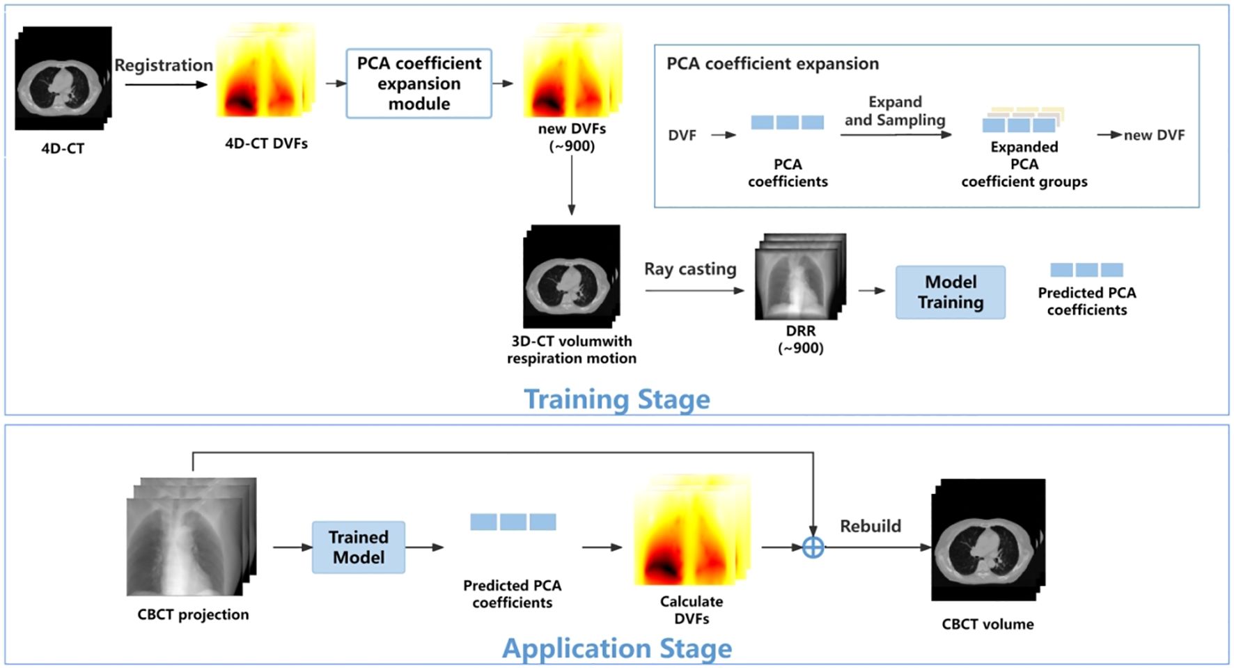
Figure 1 The workflow of the proposed method.

In the application stage, a single CBCT online projection that is measured at the same angle will be sent into the trained network. The network predicts three PCA labels to generate a phased 3D-CBCT. Then, more online projections (with different respiration amplitudes) will be continuously measured and sent into the network so that a whole respiration cycle will be covered. In this way, a full-cycle PCA label groups can be achieved and the whole 4D-CBCT. The entire process is performed on time. Below, we summarize our work into five parts: 1) motion modeling, 2) data processing, 3) network architecture, 4) loss function, and 5) experiment design.

2.1 Motion modeling

As mentioned above, the 4D-DVF is initially obtained from 4D-CT via deformable image registration (11–13). The 0% phase was selected as the reference phase to achieve the 4D-DVF. We used PCA, which is a commonly used data decoupling scheme for data dimension reduction (16), to extract DVF’s feature label (e.g., the principle components/eigenvectors). For computational efficiency consideration, we select the first three PCA labels for mapping the DVFs. Table 1 illustrates the accuracy of DVF estimation relative to the number of PCA labels used. As expected, DVF accuracy improves with an increasing number of PCA labels. However, this also increases computational complexity. We found that by using the first three principal components, it already achieved 97.22% DVF information. Further increasing the PCA labels will not dramatically increase the information anymore. Therefore, we chose to discard the remaining PCA labels in our experiment.

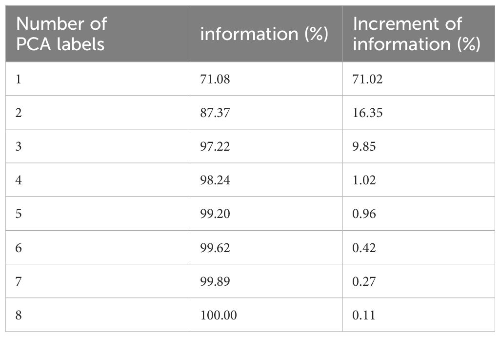
Table 1 PCA label versus DVF estimation accuracy.

The mapping relationship between the DVF and the PCA labels is given by Formula 1. Let the DVF size set be 3×NvoxelCT, where NvoxelCT stands for 3D-CT voxel number; 3 stands for the 3D motion. The DVF will be linearly mapped by Equation 1:

DVF(i)=∑j=1kpj(i)qj(i)(1)

Here, p and q stand for the eigenvectors and their corresponding PCA coefficients. Index i and j represent the respiration phase and eigenvectors, respectively.

2.2 Data processing

Being a regression task, ConvLSTM requires a large number of training data-set samples. In this study, we performed data augmentation and data enhancement. For data augmentation, we enlarged the simulated respiration amplitudes by a 15% interval up and down between two adjacent phases. This is because respiration is a time-continuous physiological motion. The concept of the 4D-CBCT phase is an average reconstruction for projections in one re-binned phase. The lung will move across the re-binned interface between two adjacent phases. Our extended motion amount covers just a bit more than the average motion range (7). This is to make sure all the possible motion amplitude will be modeled for training data generation. We perform PCA label random sampling to generate 900 DRRs as a training data set.

For data enhancement, we considered the influence of quantum noise in the simulated DRRs. Given that quantum noise is typically a combination of Poisson and Gaussian noise (17), we constructed a linear noise combination as follows see Equation 2:

N=Poisson(I0exp(−pn))+Gassian(0,σe2)(2)

pn is the noise-free signal line integral; the index N means the noise for each detector; I0 is the X-ray projection intensity; and σe2  represents background electronic noise. I0 and σe2 are set to be 105 and 10, respectively. DRR was then added to the simulated noise to achieve the real projected image.

We also implemented an intensity correction scheme to minimize the intensity mismatch between the simulated training DRRs versus the measured CBCT projections. The correction is given by Equation 3:

IDRR∧=(IDRR−IProjection)×σDRRσProjection+IDRR(3)

where IDRR∧ represents the corrected DRR intensity. IDRR  and  σDRR  represent the mean and the standard deviation of the original DRR intensity, and IProjection and σProjection represent the mean and standard deviation of measured CBCT projection.

2.3 Network architecture

We use the ConvLSTM to explore the nonlinear mapping between DRRs and the PCA coefficients. The network architecture is illustrated in Figure 2. It contains a series of ConvLSTM cells and a regression layer.

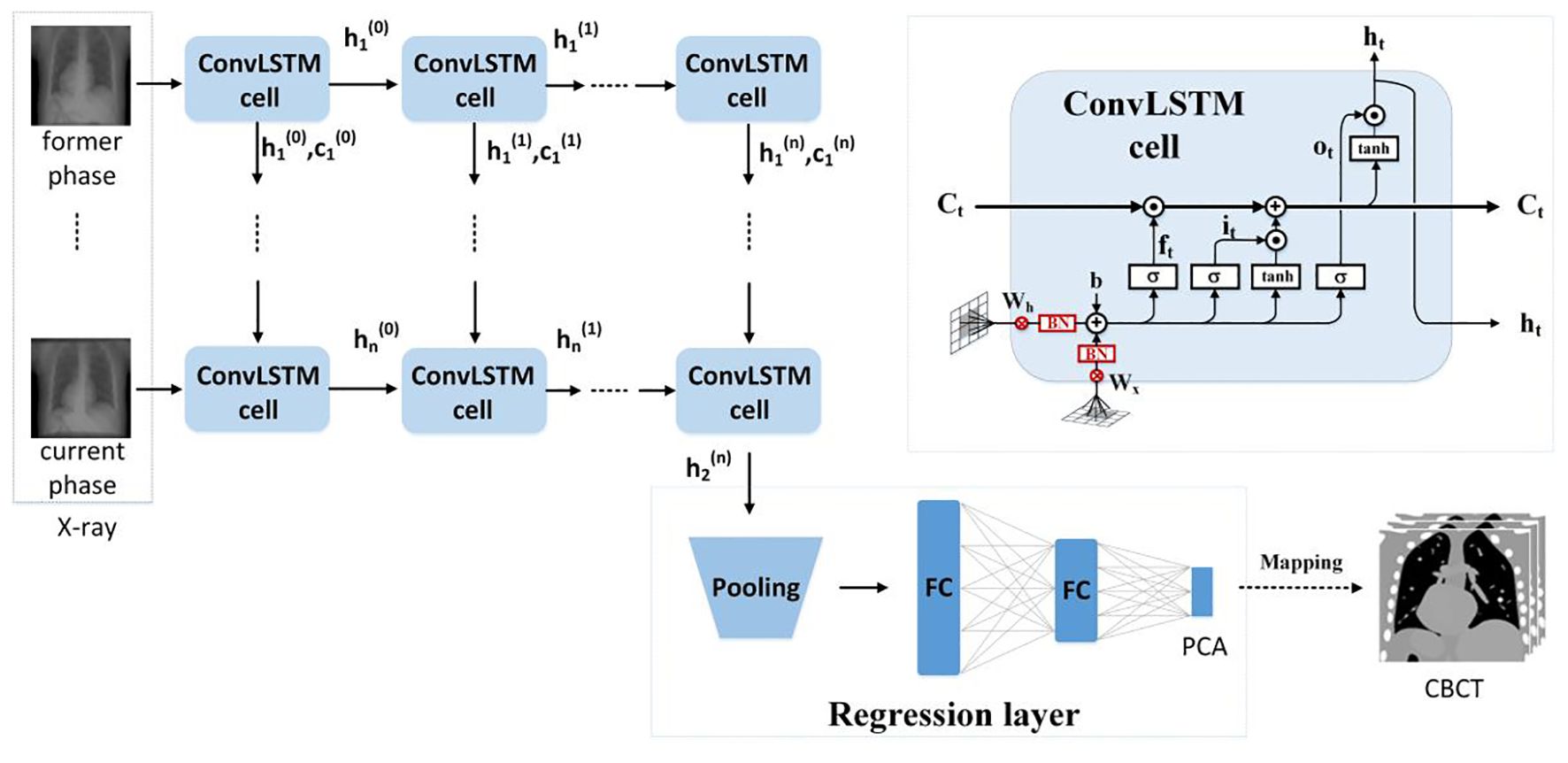
Figure 2 The ConvLSTM framework.

Conventional LSTM (18) contains a memory cell (Ct) and three gate control cells: 1) the forget grate (ft), 2) the input gate (it), and 3) the output gate (ot). Ct stores the foregone information, and the three gates update the cell. The LSTM sorts the relationships between all of the time flags; meanwhile, it ignores the internal information within each time flag. However, ConvLSTM (19), instead, explores the local features within each time flag via the convolutional operators. For the tth ConvLSTM cell, the internal operations will be represented by (19), see Equations 4–9:

it=σ(Wxi∗Xt+Whi∗Ht−1+bi)(4)ft=σ(Wxf∗Xt+Whf∗Ht−1+bf)(5)ot=σ(Wxo∗Xt+Who∗Ht−1+bo)(6)Gt=tanh(Wxg∗Xt+Whg∗Ht−1+bg)(7)Ct=ft∘Ct−1+it∘Gt(8)

σ is the sigmoid function, tanh stands for the TanHyperbolic function, ∗ and ∘ represent the convolutional operator and Hadamard product, respectively. Xt is the input of the current cell, and Gt is a candidate storage unit for information transmission. In addition, W and b denote convolution kernels and the bias terms. W and b have obvious meanings. For instance, Wxo is the input–output gate convolution kernel, while bi is the input gate bias, etc.

Due to the characteristic of the convolutional operator, ConvLSTM can acquire both temporal and spatial information simultaneously (19–22). Our ConvLSTM network contains 40 hidden layers and 20 cell layers. Moreover, it has eight layers, kernel size is 3, padding is set as “valid”, and the stride of the convolution kernel is 1.

The regression layer uses the feature map generated from ConvLSTM to predict PCA coefficients. It contains a pooling layer with two fully connected layers. By using the dominant local information, the pooling layer reduces the computation cost. The pooling was set to twice the down-sampling, and the dimensions of the two completely connected layers are 1,024 and 3.

2.4 Loss function

The normalized mean square error builds the loss function and is given in Formula 5. The PCA coefficients (e.g., output labels in the network) in the loss function (see Equation 10) ensured that the first coefficient has the highest estimation accuracy.

Loss=1N∑i=1N‖wcoeff∘(yi−G(xi,W))‖2(10)

N is the training sample number; ‖‖2 represents the L2 norm, and o is the element-wise product. G(xi,W) is the output of the regression model. xi is the ith training image, yi is the PCA coefficient, and W is the network parameters. wcoeff is the PCA coefficients weight, which is set to be [26,16,16].

For model training, the ADAM optimizer was utilized with a dynamic learning rate, initially set at 0.001. The batch size was set to 8, and the training ran for 200 epochs. In an environment configured with Python 3.7 and an NVIDIA GeForce RTX 4080, training the data for 200 epochs took approximately 36 h.

2.5 Experiment design

For network performance evaluation, we use XCAT phantom and patient 4D-CT for the quantification. For testing, we simulated an on-board CBCT projection and then sent it into the pre-trained network to predict PCA coefficients. The quantification evaluation labels that we used are 1) the Mean Absolute Error (MAE), 2) the Normalized Cross Correlation (NCC), 3) the Multi-scale Structural Similarity(SSIM), 4) the Peak Signal-to-Noise Ratio (PSNR), 5) the Root Mean Squared Error (RMSE), and 6) the Absolute Percentage Error (MAPE). MAE is used to quantify the accuracy of regression models. y and y^ represent the label and the predicted value of the model, and i stands for the index of the regression model. We have in Equation 11:

MAE=1m∑i=1m|y^(i)−y(i)|(11)

In addition, NCC and SSIM (Multi-scale Structural Similarity Index Measure) are used to evaluate the quality of the reconstructed image. See Equations 12 and 13. S and T represent slice data with size of H×W of the original image and the reconstructed image, respectively. μ, δ, and δ2 represent the mean, covariance, and variance of the slice image, respectively.

NCC=∑k=1C∑i=1H∑j=1W|S(i,j)−μs||T(i,j)−μT|C∑i=1H∑j=1W(S(i,j)−μs)2(T(i,j)−μT)2(12)SSIM=(2μsμT+C1)(2δST+C2)(μs2+μT2+C1)(δS2+δT2+C2)=l(s,T)·cs(s,T)(13)

PSNR is defined based on MSE (Mean Squared Error). See Equations 14 and 15:

MSE=1N∑j‖S(j)−T(j)‖2(14)PSNR=10∗loɡ10MAX2MSE(15)

N is the image pixel number. MAX is the maximum possible pixel value.

The definition of RMSE is given in Equation 16:

RMSE=∑i=1M∑j=1N(Sij−Tij∗)2H×W(16)

MAPE is the average ratio of the absolute difference between the predicted value and the true value to the true value. The definition of MAPE is given in Equation 17:

MAPE=1n∑j|Sj−TjTj|(17)3 Results3.1 Network parameter optimization

Being a spatiotemporal sensitive network, the temporal continuous image amount that the network can handle for data training reflects its ability for accurate motion estimation. However, Figure 3 indicates that the model prediction accuracy is not dramatically influenced by the input image number. The MAE values fluctuate between 47 and 57, and the SSIM remains approximately 0.93. We found that the model achieves the best performance with four continuous temporal images with the lowest MAE of 47.15 and highest SSIM of 0.95.

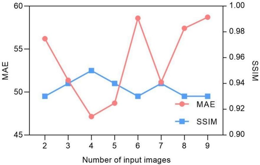
Figure 3 Input image quantity vs. MAE/SSIM of model prediction.

The selection of hyper-parameters for the ConvLSTM network was a critical aspect, as these parameters significantly impact the prediction performance of the model. To determine the optimal configuration, we conducted a series of ablation experiments focusing on the number of hidden layers and cell layers within the ConvLSTM network. The experiment results in Figure 4 reveal that increasing the number of hidden layers decreased the MAE without significantly affecting computation time, although it did increase the number of parameters. Conversely, increasing the number of cell layers resulted in a slower decrease in MAE and an increase in computation time, with little change in parameter count. By balancing these factors, we determined that a configuration with 40 hidden layers and two cell layers provided the optimal trade-off, ensuring high prediction accuracy while maintaining computational efficiency.

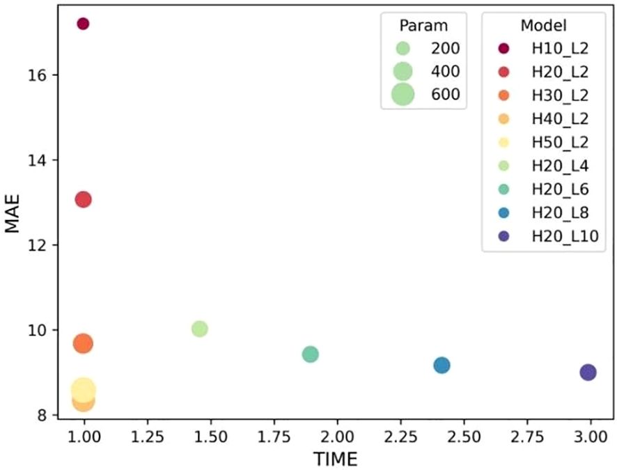
Figure 4 Influence of ConvLSTM cells on the model’s prediction. “H” stands for the number of hidden layers; “L” denotes the number of cell layers.

3.2 Convergence of loss function

The convergence of the loss function is decided by the weightings. Table 2 shows the convergence comparison caused by different weightings. Their MAE and NCC values are also summarized in the table. We found that the second group weighting (e.g., [2/6, 1/6, 1/6]) has the smallest first PCA label error. Meanwhile, this group also got the highest NCC.

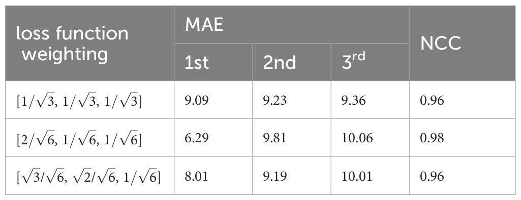
Table 2 Weighting influence on MAE/NCC.

Suitable choice of the pooling will also speed up loss function convergence. See Figure 5. The figure compared loss convergence curve with epoch with different pooling scheme such as Maximal pooling, Converlutional pooling, average pooling, and even no pooling at all. The results show that convolutional pooling achieves the best convergence performance. The pooling operation reduces the model’s parameters, hence accelerating its convergence.

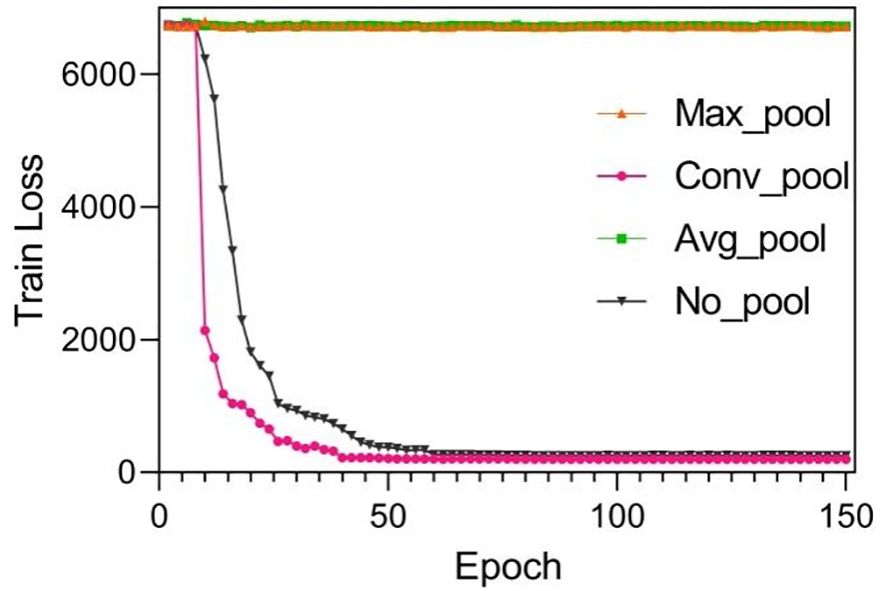
Figure 5 Training results by using different pooling optimizations. These pooling operations are set to twice the down-sampling, and the model only performs a single pooling operation.

Suitable choice of pooling will also speed up loss function convergence. Figure 6 compares the loss convergence curve with different pooling schemes such as maximal pooling, convolutional pooling, average pooling, and even no pooling. The results show that convolutional pooling achieves the best convergence performance. The pooling operation reduces the model’s parameters, hence accelerating its convergence.

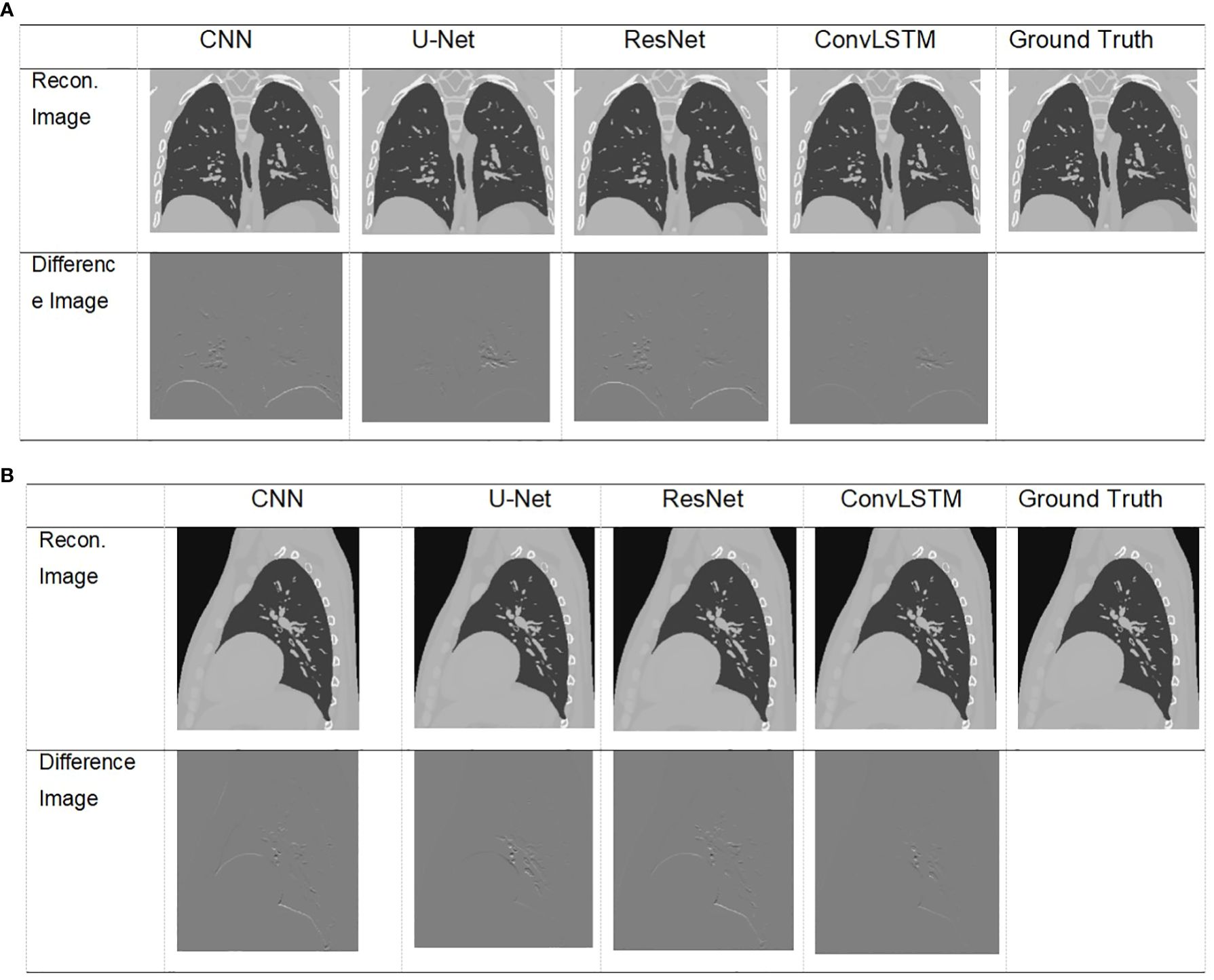
Figure 6 Visualization of images result of TestCase1 in different anatomical surfaces for each model with the training data generated from XCAT. (A) Coronal plane; (B) sagittal plane.

3.3 XCAT simulation results

The XCAT phantom-based digital experiment was first performed. Four state-of-art network structures (e.g., CNN/Unet/ResNet/ConvLSTM) were tested with the phantom to compare their performances. As shown in Table 3, for the two test cases, the ConvLSTM outperforms other models in PCA coefficient prediction, especially for the first coefficient. The bold values provided in Table 3 means that ConvLSTM achieves the best PCA coefficient match compared with that of the ground truth for XCAT phantom. By utilizing PCA to reduce the dimensionality of the DVFs, the ConvLSTM network focuses on the most significant components of respiratory motion. This not only improves computational efficiency but also ensures that the network is learning the most relevant features for accurate motion prediction. Figure 6 presents the reconstructed results based on the PCA coefficients predicted by ConvLSTM versus CNN/UNet/ResNet. The reconstructed coronal plane and sagittal plane images and the different images between each reconstruction and the ground truth image are summarized in Figures 6A, B.

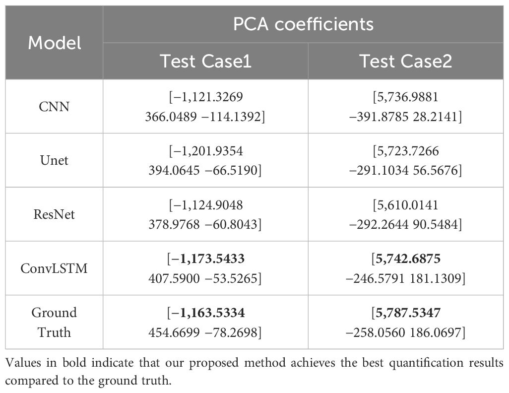
Table 3 Comparison of prediction results versus ground truth of XCAT data.

Table 4 summarizes the quantification evaluation comparison between each network. The results indicate that ConvLSTM outperformed other networks for all of the evaluation labels.

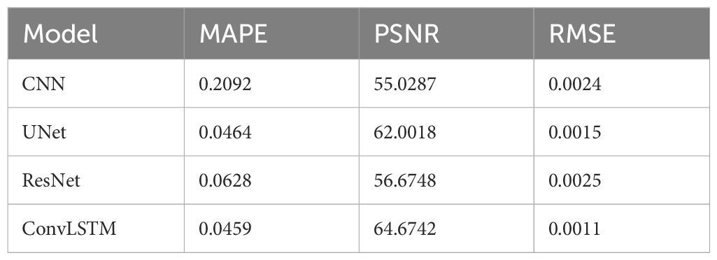
Table 4 Quantification comparison of prediction and reconstruction of each model on the coronal plane in XCAT TestData1.

3.4 Pilot clinical results

Table 5 shows two cases of the real and predicted first three PCA coefficients of the patient data results. It is well known that the higher the principal component order, the higher the PCA contribution rate. As can be seen from Table 5, the first principal component of the model based on ConvLSTM is closest to the true value, just as the bold values illustrated. Figure 7 shows the reconstructed coronal images based on the PCA coefficients predicted by CNN/UNet/ResNet and ConvLSTM network. We can see that all models have successfully recon