Random utility theory for paired comparisons

The theoretical framework of this choice analysis is based on random utility maximization (RUM) theory. According to RUM theory, the utility function \(_=_+_\) of individual \(i=1,\dots N\) for alternative \(j=1,\dots ,J\) in choice situation \(t=1,\dots T\) can be decomposed into a deterministic part of utility \(_\) (representative utility) and a random part of utility \(_\). In paired comparison modeling [10], individual \(i\) will choose an alternative \(j\) if and only if the probability that the utility associated with alternative \(j\) is higher than the utility of its alternative.

$$\begin_=P\left(_>_ \right), \forall \,k\ne j\\ _=P\left(_+_>_+_\right), \forall \,k\ne j\\ _=P\left(_-_<_-_ \right), \forall \,k\ne j\end$$

(1)

Choice probabilities are calculated based on a relative measure where the utility of one of the alternatives in the choice set is taken as a reference. To derive the choice probabilities, we need to make distributional assumptions about the random part of utility. The conditional logit (CL) model is derived under the assumption that \(_\) is independently and identically distributed (IID) with an extreme value type I (EV1) distribution [11,12,13]. As a result, the difference between two IID EV1 random error terms \(_-_)\) has a logistic distribution with scale parameter \(\lambda\). This implies that the choice probabilities of the CL model can be expressed in terms of a logistic distribution with a cumulative distribution function

$$}}_}}}}=\frac}=1}^}}\text[}(}}_}}}}-}}_}}}})]},\boldsymbol\forall \,\boldsymbol}\ne }$$

(2)

where \(\lambda\) is the scale parameter [14].

Scale and rate heterogeneity in health valuation

For this study, we extended the CL model (Eq. 2) for health valuation on a quality-adjusted life-year (QALY). By construction, the scale parameter is always positive, \(\lambda =\text(\mu )\), and represents the relationship between log-odds and the value of a health outcome \(_\) on a QALY scale. We specify the value of a health outcome \(_\) as a product of two values representing heath \(_^\) and life years \(_^\):

$$}}_}}}}=}}_}}}}^}}\times }}_}}}}^}}$$

(3)

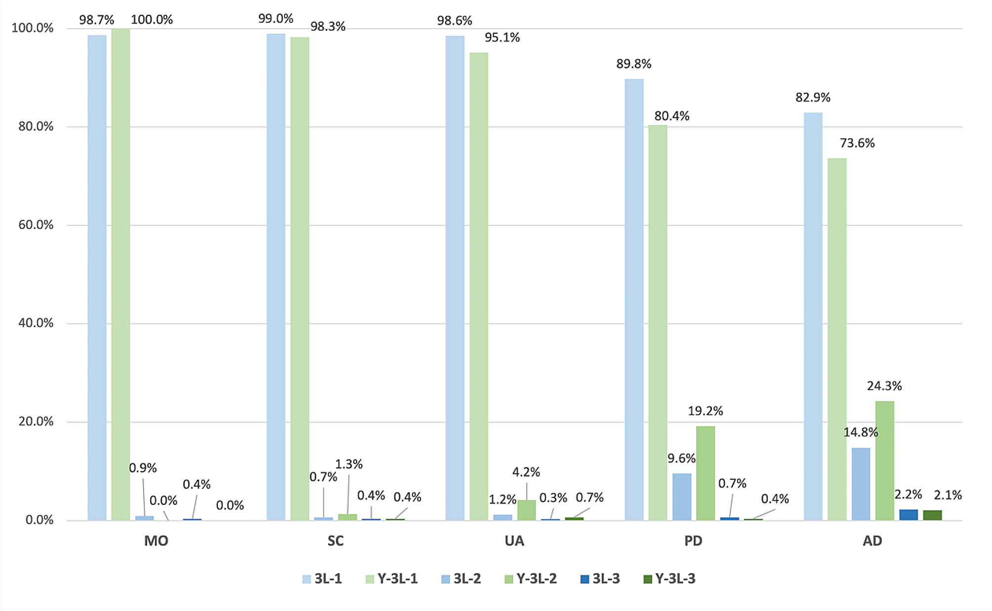
In this paper, we assume that the value of health \(_^=1-x}_\), where \(_\) is a vector of 20 incremental indicators of health problems in mobility, self-care, usual activities, pain/discomfort and anxiety/depression (i.e., MO, SC, UA, PD, AD), and \(\beta\) is a vector of preference weights on a QALY scale. Its homogeneity is a simplifying assumption for the estimation of a single EQ-5D-5L5L value set that may be relaxed in future work.

More specifically, the value of the health profiles is parameterized using 20 incremental effects (i.e., 5 attributes with 4 levels each), where each effect is caused by a dummy variable representing an incremental change in the level of severity of an EQ-5D-5L attribute. Therefore, we can write

$$_^=1-\left(\begin\begin_M_+_M_+_M_+_M_+\\ _S_+_S_+_S_+_S_+\\ _U_+_U_+_U_+_U_+\end\\ _P_+_P_+_P_+_P_+\\ _A_+_A_+_A_+_A_\end\right)$$

(4)

As a criterion of face validity, all 20 incremental effects in vector \(\beta\) should be positive since they represent losses in value due to increases in the level of severity of a health condition from the full health profile [14].

For the value of life years \(_^\), the identity function is commonly assumed to be \(_^=_\), where \(_\) represents life years (i.e., no discounting). However, this functional form does not accurately represent the time preferences of the general population [4, 5]. Individuals usually discount over time; i.e., future outcomes affect choices less than present outcomes. To allow for temporal discounting, we adapt the power function (see 4)

where \(_\) is the individual-specific power. On a QALY scale, the value of time \(_^\) equals 1 when \(_\) equals 1, regardless of the power \(_\), and the identity function (i.e., no discounting) implies that the power is unity, \(_=1\).

Apart from restricting the individual-specific scale parameter to be positive, \(_=\text(_)\), we restricted the power \(_\) to the unit interval, \(0\le _\le 1\). More specifically, we transform the power into a discount rate using the complementary log–log (CLL) function, \(_=\text(-\text\left(_\right))\) which is naturally bounded to the unit interval. At first glance, \(_\) has an inverse relationship with \(_\), and a lower \(_\) implies greater discounting of life years; therefore, a higher rate \(_\) implies greater discounting. Future analyses may allow for negative discounting or alternative functional forms [15,16,17].

The bivariate distribution of the scale and rate among respondents

Due to limited panel evidence per respondent, it is not feasible to estimate individual-specific scales and rates as fixed effects (i.e., \(_\) and \(_\)). Instead, we estimated a conditional logit (CL) model and three mixed logit models. First, we estimated the CL model under homogeneity \((_=\mu ; _=r)\). Under this specification, all respondents have the same scale parameter and discount rate. In the second and third specifications, we estimated the mixed logit models with random scale and random rate, respectively. We refer to these two mixed logit specifications as “univariate” models because each contains only one normally distributed random parameter.

Finally, in the fourth specification, we estimated a bivariate mixed logit model, including the mean and standard deviation of \(_\) (i.e., \(\mu\) and \(_\), respectively) and \(_\) (i.e., \(r\) and \(_\), respectively), as well as their correlation. The ancillary parameters vary under a bivariate normal distribution and may be correlated. We assume that \(_\) and \(_\) are normally distributed such that \(\left(_,_\right)\sim N(_^,\rho ,_^)\) where \(_^=Var(_)\), \(_^=Var(_)\) and \(\rho =Corr(_,_)\).

To shed more light on this potential bias, we express the individual-specific ancillary component, \(__^\) (apart from the value of health), as an exponential regression with two ancillary parameters (an intercept \(_\) and a coefficient \(_)\), where \(_>0:\)

$$__}^=\text\left(_\right)_^_}=\text\left(_+_ln\left(_\right)\right)$$

In this study, life years \(_\) range from 1 to 10 years; therefore, \(ln\left(_\right)\) ranges from zero to 2.303. Given that \(ln\left(_\right)\) is always positive, the ancillary component can increase through either ancillary parameter (\(_\) or \(_\)). In econometric terms, \(ln\left(_\right)\) is an instrumental variable needed to identify the two ancillary parameters.

Data

In 2016, 8,222 U.S. respondents (4074 in wave 1 and 4148 in wave 2) from all 50 states and Washington, D.C., completed an online survey that included 20 paired comparisons. The design of the paired comparisons was largely based on the EuroQol Valuation Technology (EQ-VT v1.0) protocols [18]. An example of the paired comparison conducted in the study is illustrated in Fig. 1. In this paper, we provide a general overview of the study. More details can be found in other studies [3, 19].

Fig. 1

Example of a paired comparison

Each paired comparison is presented as a variation of health descriptions based on the EQ-5D-5L. The five dimensions (i.e., attributes) of the EQ-5D-5L are mobility, self-care, usual activities, pain/discomfort and anxiety/depression, where each dimension is characterized by five levels ranging from no problems (i.e., level 1) to slight, moderate, severe, and unable/extreme problems (i.e., level 5). For instance, the health description on the right side of Fig. 1 can be represented as a vector of five numbers 33333 since all five dimensions are at a moderate level. For each comparison, respondents were asked, “Which do you prefer?” regarding a pair of alternatives described using the EQ-5D-5L and lifespan attributes.

The online survey consisted of 3160 pairs, 1600 of which are efficient (or “quality only”) pairs and 1560 of which are quantity-quality pairs. In efficient pairs, both health descriptions consisted of varying levels of health problems with the same life years (e.g., 12345 vs 54321). In the quantity-quality pairs, one of the health descriptions involves no health problems (i.e., 11111). Furthermore, 80 out of 1560 quantity-quality pairs included “immediate death”, which represents “dead” pairs, as one of the alternatives. The data were collected in two parts: an exploratory survey consisting of 1560 pairs and a confirmatory survey consisting of 1600 pairs. The survey data were collected at four temporal units (i.e., days, weeks, months, and years). This analysis included only the pairs with year units (1017 respondents in wave 1 and 1229 in wave 2) because the other pairs did not describe events after 1 year (i.e., discounting).

With the diversity of pairs, it is mathematically feasible to identify the scale and rate separately using either wave of this dataset. Imagine a paired comparison with identical lifespans. These pairs may identify differential scales within a population, \(_\). Imagine a paired comparison with differential life years. These pairs may identify differential scales, \(_\) and rates, \(_\). Apart from its pair types, this dataset is one of the largest national health valuation studies ever conducted [3], has both exploratory and confirmatory waves, and applied quota sampling at the pair level to assure that each pair had a minimum number of respondents along 18 demographic quotas.

Mixed logit and maximum simulated likelihood

To estimate the mixed logit models, the maximum likelihood (ML) estimator of parameter vector \(\theta\) can be utilized when the density of dependent variable \(_\) conditional on a vector of independent variables \(_\), \(f(_|_,\theta )\), has a closed-form such that

$$}_=\text\underset}_^\textf(_|_,\theta )$$

where \(i=1,\dots ,N\). However, ML is not feasible when \(f(_|_,\theta )\) does not have a tractable closed-form. This can be because the density is specified only conditional on latent variables, which cannot be integrated out. Thus, the MSL estimator is a possible alternative [20, 21]. Suppose \(\widetilde(_,_,_,\theta )\) is an unbiased simulator of the conditional density \(f(_|_,\theta )\) such that

$$f\left(_|_,\theta \right)=}_}[\widetilde(_,_,_,\theta )|_,_]$$

where \(_\) is an individual-specific latent vector (\(_\) and \(_\)) whose distribution is known and independent of \((_,_)\). Then, the MSL estimator of \(\theta\) is defined as

$$}_=\text\underset}\sum\limits_^\text\left[\frac\sum\limits_^\widetilde(_,_,_^,\theta )\right]$$

where \(_^(s=1,\dots ,S)\) are drawn independently for each individual \(i\) from the distribution of \(_\). The MSL estimator is obtained by replacing the intractable conditional p.d.f. \(f(_|_,\theta )\) with its unbiased approximation based on the simulator \(\widetilde(_,_,_^,\theta )\). In this study, we estimate the mean and variance of each random parameter as well as their p-values [3].

In our MSL estimations of the three specifications of the mixed logit model, we use 250 Halton draws (i.e., \(S=250\)) [22]. We used the MATLAB programming language for all estimations. More specifically, we began by estimating the CL comparator and three specifications using the wave 1 data, which helped us state our hypotheses more clearly. Afterwards, we re-estimated the models and tested these hypotheses using the wave 2 data. Furthermore, we compare the results between waves and models to assess how allowing heterogeneity in scale and rate affects the estimation of EQ-5D-5L values.