An observational and prospective study was carried out with 110 patients. The patients were recruited consecutively in general gynecology consultations from 1 April 2023, to 31 July 2023. Patients did not need to suffer from pelvic floor pathologies to qualify. However, patients who underwent surgery or had a history of pelvic floor dysfunction and patients with problems that made it difficult to perform a correct Valsalva maneuver were excluded. All patients were gynecologically evaluated before being included in the study to rule out pelvic floor dysfunction. The clinical parameters studied were age, weight, height, body mass index (BMI), parity, menopausal status, and age at menopause.

The transperineal ultrasound scans were performed by an expert pelvic floor sonographer on a Canon i700 Aplio® (Canon Medical Systems, Tokyo, Japan) with a PVT-675 MV 3D abdominal probe. The images were acquired with patients in the dorsal lithotomy position with their hips flexed and following the guidelines previously established in the literature [1]. The probe (covered with a protective sleeve) was carefully placed in the perineum, less than 1 cm from the pubic symphysis, with both labia minora on the sides of the transducer. The midsagittal plane included a view of the symphysis pubis, urethra, bladder, vagina, uterus, anus, rectum, and levator ani muscle. To obtain a good image of the uterine fundus, low frequencies were used to capture a complete image of all the organs. The orientation of the ultrasound videos was established such that the cranioventral region was on the left and the dorsocaudal region was on the right (Video 1) [9]. Before the video was captured and stored, the patient was trained to perform the Valsalva maneuver correctly. A video was made of each patient that included the midsagittal plane of the pelvic floor at rest and the change in the pelvic structures during the Valsalva maneuver. After saving the captured videos, we manually labeled the different organs in each video (Video 1). Labeling was performed by correcting the movement of the different organs during the Valsalva maneuver (Video 1). Tagging was performed by two independent scanners and supervised by an expert scanner (JAGM).

Data were labeled using the free software CVAT, developed by Intel specifically for annotating both images and videos. CVAT offers a variety of annotation shapes and types, including labels, bounding boxes, polygons, polylines, dots, and cuboids.

For each video, the sonographer selected a series of frames based on observable changes in the image resulting from patient maneuvers. These frames were annotated by outlining polygons around each organ of interest. As only a subset of frames was annotated, labels for the remaining frames needed to be provided. In this study, linear interpolation between two adjacent annotated frames was used to generate labels for the remaining frames.

A total of 110 videos were tagged and randomized into two groups. The first group comprising 86 tagged videos served as the CNN training set, whereas the second group of 24 videos was used for CNN validation.

Prior to training the networks, the ultrasound images were preprocessed to eliminate the background, converted to grayscale and resized to 128 × 128 pixels. The data were input into the network in their raw format. No preprocessing was applied to the images to remove noise or to adapt to the variability of the distributions. Instead, these tasks were delegated to the neural network.

In total, 15,932 raw images (before applying data augmentation preprocessing) were distributed across the training, validation, and test sets. Data splitting was performed on a per-patient basis to mitigate the risk of overfitting. This approach ensures that the model generalizes well to unseen patient data, thereby enhancing the reliability of the results.

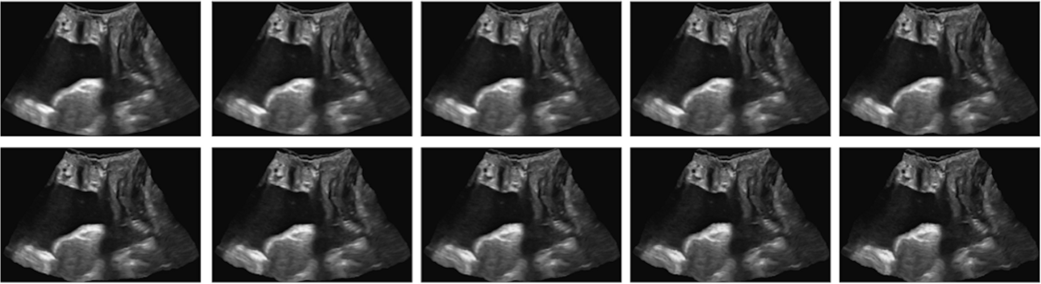
Various data expansion techniques, including rotation, scaling, translation, and elastic transformations, were tested. The rotation range applied was between −180 and 180°. The scaling factor ranged between 0.8 and 1.5, and the translation sliding was 10% from the center of the image in all directions. These ranges were applied randomly. Figure 1 shows an example of the elastic transformations applied to a video frame.

An example of the elastic transformations applied to a video frame

In this work, three different architectures were tested: UNet, FPN, and LinkNet (Fig. 2). These architectures are well-known models utilized for image segmentation tasks. They were selected to evaluate their performance on 2D ultrasound images in the midsagittal plane, with the aim of estimating the regions of eight different organs. UNet [10] was designed expressly for segmenting medical images and has been used extensively in this context. It comprises two parts: an encoder and a decoder. The encoder performs a dimensionality reduction in which it extracts the useful feature information that will be used by the decoder. In this phase, as the network deepens, the spatial information is reduced. The decoder performs a dimensional expansion in which characteristic information is combined with spatial information to construct the output. These connections between the encoder and decoder are known as skip connections. LinkNet [11] has a very similar structure to UNet, except that a sum operation is applied in the connections between the encoder and decoder. This difference, such as the use of separable convolutions and 1 × 1 convolutions, achieves better computational efficiency and training speed and maintains good performance in segmentation precision. Finally, the feature pyramid network (FPN) [12] reuses the feature maps of each stage of the decoder to concatenate them after unification of the dimensions and to obtain the final segmentation.

Three different architectures were used. A UNet architecture with skip connections that use concatenation. B LinkNet, in which the sum operation is used in skip connections. C FPN shows the validation for the selection of the best network. D Data partitioning, cross-validation, and final training methodology. E Model performance during training on the validation sets of each fold. The green vertical line indicates the best average performance obtained

For each architecture, 11 different backbones were tested (ResNet50, VGG16, VGG19, DenseNet121, BeingsNet50, ResNeXt50, BeingsNeXt50, Inceptionv3, InceptionResNetv2, EfficientNetv5, and EfficientNetv7). The backbone is a network that is used as an encoder and that can be pretrained. In this work, the weights of the backbones were randomly initialized.

To avoid possible overfitting when selecting the best network, cross-validation was applied (Fig. 2). Five folds were used; thus, the model was trained on 69 cases and validated on 17 cases. As a criterion for stopping the training, early stopping was used with a stopping criterion of five times without improvement in the mean of the validation errors of the five folds. In total, 165 networks were trained (3 networks × 11 backbones × 5 transformations).

The networks were trained with a cost function (loss function) that combines the focal function with the Dice function. The Dice function, which measures the level of overlap of the prediction and the labeled region, assigns a weight of 1 to the region of each recognized organ and a weight of 0.5 to the background. The focal cost function [13] is an improvement of the cross-entropy function to address unbalanced data and focuses more on samples that are difficult to classify.

Figure 3 displays the results for each architecture compared with each backbone and the data augmentation applied. The best model was found to be FPN + ResNet50, with elastic transformations at a probability of 50% (the elastic transformation was applied to 50% of the training samples). This model was trained with 86 cases for the number of epochs determined by the stop criterion via cross-validation.

The graph compares the validation and test Dice Similarity Index scores obtained for each pair of network architecture and backbone with a specific data augmentation

The model was trained to independently estimate the region of each organ in every frame. Once trained, the model was applied to predict all frames within the test videos, and the scores are computed by measuring the mean performance per video.

All networks were trained using an NVIDIA GTX 1080Ti GPU installed on an Intel Core i5-7500 3.40 GHz CPU running Ubuntu 20 with 32 GB of RAM. To implement the networks, the Keras framework and the segmentation models package were used [14].

The Dice Similarity Index (DSI) was used for CNN validation. The DSI determines the similarity between manual labeling and the CNN; a DSI = 0 indicates no overlap between the manual segmentation and the CNN, whereas a DSI = 1 indicates maximum overlap between the segmentations. The DSI is calculated using the following formula: (2 | X ∩ Y |) ÷ (| X | +| Y |), where X and Y are the two segmentations. In addition, the intersection over union (IoU) was used, which describes the level of overlap between two boxes, that is, the prediction box and the real bounding box. The greater the overlap, the greater the IoU. The IoU is calculated by determining the Jaccard index: IoU = (ANB) ÷ (AUB) or (I) ÷ (U).

An expert observer (JAGM) compared the manually tagged videos with the CNN segmentations of the 24 videos used for validation. The expert observer considered the image to be correctly recognized by the CNN when its segmentation completely identified the organ under study; that is, the segmented image was similar to the image that was manually labeled (Video 1). A CNN segmentation that partially identified the organ (Fig. 4) or a segmentation image that was different from the image that was manually labeled (Fig. 4) was classified as incorrect.

The image shows correct recognition (A) and defective recognition (B) of the different organs of the pelvic floor in the midsagittal plane by the convolutional neural network according to the expert explorer. In B there is a partial lack of recognition of the urinary bladder owing to the pubic shadow (1) and poor delimitation of the posterior uterine surface owing to the similar echogenicity that the uterus can present with the intestinal loops (2). Box plot showing the general Dice Similarity Index (DSI; DICE) and the DSI of the different organs (C)

Statistical analysis was performed using the IBM SPSS Statistics version 26 program (IBM, Armonk, NY, USA). The data were reviewed before statistical analysis. To describe the numerical variables, means and standard deviations (SDs) were used in the case of an asymmetric distribution. For example, the medians and percentiles (p25 and p75) were used, and the qualitative variables were expressed as percentages.

The study was conducted in accordance with the Declaration of Helsinki (as revised in 2013). The study (0625-N-23) was approved by the local Ethics and Research Committees in April 2023. All patients provided written informed consent before starting the study.