Study participants

Patients with episodic migraines were recruited from an academic headache clinic between October 2020 and November 2021. The inclusion criteria for patients were: (1) age 18–50 years; (2) not taking preventive medications; and (3) premenopausal status in female patients. The exclusion criteria included: (1) chronic migraine, medication-overuse headaches, chronic pain disorders other than migraine, and psychiatric disorders such as bipolar affective disorder or schizophrenia; (2) contraindications for 3T MRI, including use of a tissue expander, pacemaker, non-detachable metal objects, orthodontic devices, or electrical leads or implants in the body; (3) pregnancy; (4) claustrophobia requiring sedation during MR scanning; (5) inability to report their headache or complete the headache diary due to cognitive decline; and (6) disagreement with the study procedures. Migraine was diagnosed according to the ICHD-3 criteria by a single investigator (MJL), a neurologist specializing in headaches. This study was approved by the Samsung Medical Center Institutional Review Board, and all participants provided written informed consent to participate. This study was part of an ongoing longitudinal project registered at ClinicalTrials.gov (NCT03487978).

MRI data acquisition

T1-weighted structural and diffusion MRI data were obtained using a Philips Ingenia 3T scanner (Philips, Amsterdam, Netherlands). T1-weighted data were acquired using a turbo field echo sequence in the sagittal plane (repetition time [TR] = 8.1 ms; echo time [TE] = 3.7 ms; field of view [FOV] = 256 × 256 mm2; voxel size = 1 mm isotropic; and number of slices = 180). Diffusion MRI data were acquired using a spin-echo echo-planar imaging sequence in the axial plane (TR = 7,062 ms; TE = 91 ms; FOV = 220 × 220 mm2; voxel size = 1.719 × 1.719 × 3 mm3; number of slices = 47; b-value = 1,000 s/mm2; number of diffusion directions = 64; and number of b0 images = 1). T1-weighted MRI scanning was performed for 3 min 20 s, and diffusion MRI for 7 min 50 s.

MRI data preprocessing

The T1-weighted MRI data were preprocessed using the fusion of neuroimaging preprocessing (FuNP) surface-based pipeline [16], which included gradient nonlinearity correction, non-brain tissue removal, and intensity normalization. The cortical surfaces were generated using FreeSurfer v7.1.1 (Boston, MA, USA) [17] by following the boundaries between the white and pial surfaces [18,19,20]. The mid-thickness surface was generated by averaging the white and pial surfaces, and was used to generate an inflated surface. Diffusion MRI data were preprocessed using MRtrix3 v3.0.2 [21], including denoising, Gibbs ringing artifact removal, susceptibility distortion correction, head motion correction, and eddy current correction. Anatomically-constrained tractography was further performed using different tissue types of the cortical and subcortical gray matter, white matter, and cerebrospinal fluid, as defined using T1-weighted MRI [22]. T1-weighted and diffusion MRI data were co-registered using FSL v6.0 [23], and different tissue types were transformed into the native diffusion MRI space. After estimating the single-shell response functions [24], constrained spherical deconvolution and intensity normalization were subsequently performed [25]. A tractogram was further generated using a probabilistic approach with 40 million streamlines [26, 27]. Options were set with a maximum tract length of 250 and a fractional anisotropy cutoff of 0.06. Spherical deconvolution-informed filtering of tractograms (SIFT2) was further applied to reconstruct the whole-brain streamlines weighted by cross-section multipliers [28]. The structural connectivity matrix was constructed by mapping the reconstructed cross-section streamlines onto a sub-parcellation of the Desikan–Killiany atlas with 300 parcels [29]. The sub-parcellation of the Desikan–Killiany atlas was defined in MICAPIPE (https://github.com/MICA-MNI/micapipe/tree/master/parcellations) [30], which subdivided the FreeSurfer segmentation into several sub-regions.

Structural connectivity gradient generation

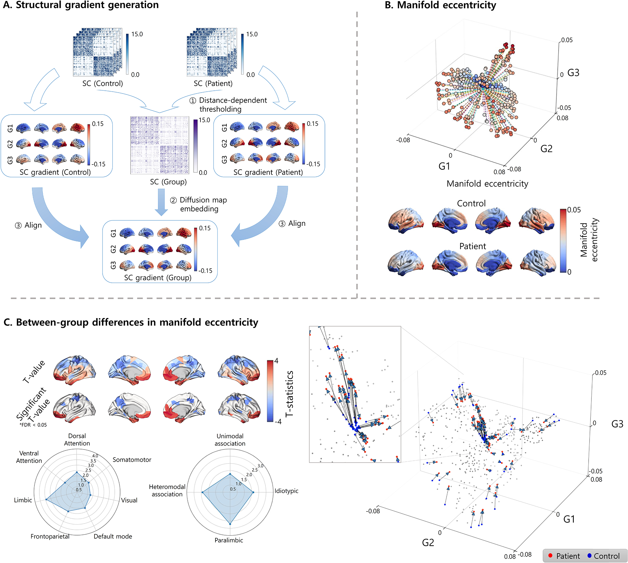
We generated low-dimensional representations of structural connectivity (i.e., gradients) by applying manifold learning, a nonlinear dimensionality reduction technique [10]. The application of manifold learning to high-dimensional data allows the generation of multiple low-dimensional eigenvectors to construct a newly defined low-dimensional space (i.e., a manifold space). First, we constructed a group representative matrix computed using distance-dependent thresholding to preserve long-range connections [31]. Using the BrainSpace toolbox (https://github.com/MICA-MNI/BrainSpace [10]), we then applied diffusion map embedding, a robust and computationally efficient nonlinear dimensionality reduction technique [32, 33], to the group-representative structural connectivity matrix. Individual gradients were estimated by applying diffusion map embedding to the individual structural connectivity matrix and were aligned to group representative gradients using Procrustes alignment [10, 34].

Manifold eccentricity and between-group differences

We subsequently generated three structural connectivity gradients that sufficiently explained total connectivity information and showed biologically interpretable axes [15, 35, 36]. Multiple gradients were further summarized into a single feature termed manifold eccentricity, defined as the Euclidean distance between each data point and the center of the data in the manifold space [15]. Differences in manifold eccentricity between patients with migraines and healthy controls were assessed using non-parametric permutation tests. The subject indices were randomly shuffled, and an analysis of covariance (ANCOVA) was performed by controlling for age and sex. This process was repeated 10,000 times. A null distribution of the between-group differences was constructed, and the p-value was calculated by dividing the number of absolute permuted statistical values larger than absolute value of the real statistic by the number of permutations. Multiple comparisons across brain regions were corrected using a false discovery rate (FDR) < 0.05 [37]. To quantify the between-group difference effects on manifold eccentricity according to brain networks, we further summarized the statistical values according to seven intrinsic functional communities, including the visual, somatomotor, dorsal attention, ventral attention, limbic, frontoparietal, and default mode cortices [38], and cortical hierarchical levels, including idiotypic, unimodal association, heteromodal association, and paralimbic areas [39].

Changes in subcortical structures

In addition to investigating the changes in cortical manifold eccentricity, we further assessed the between-group differences in subcortical structural connectivity by analyzing the degree of subcortico-cortical structural connectivity, defined as the sum of edge weights connecting each subcortical region to all cortical regions. The subcortical structures of the thalamus, caudate, putamen, pallidum, hippocampus, amygdala, and accumbens were defined from the T1-weighted data using FSL FIRST [40]. We further conducted 10,000 permutation tests, and multiple comparisons across the subcortical structures were corrected using an FDR threshold of < 0.05.

Classification between patients with migraine and healthy controls

To validate the above features, we adopted supervised machine learning to classify patients with migraines and healthy controls using the cortical manifold eccentricity and degree values of subcortico-cortical connectivity. Specifically, following the regression of age and sex from the features, we applied the least absolute shrinkage and selection operator (LASSO) method to select the imaging features [41], and entered the selected features into a linear regression model. We further performed the classification task using a five-fold cross-validation framework by dividing the data into training (4/5 partitions) and testing (1/5 partitions) datasets. The procedure was repeated 100 times using different training and testing datasets to avoid subject selection bias. Classification performance was assessed using precision, recall, and area under the receiver operating characteristic (ROC) curves (AUC), and the mean scores with standard deviation (SD) across 100 repetitions were reported.

Sensitivity analysisA) Excluding patients with migraine with aura

To evaluate the impact of migraine with or without aura on between-group differences between patients with migraine and healthy controls, we further assessed the differences in the manifold eccentricity and degree values of subcortico-cortical connectivity after excluding patients with migraine who had an aura (n = 7).

B) Different parcellations

To assess the robustness of the findings across different spatial scales, we repeated the analyses using a sub-parcellation of the Desikan–Killiany atlas with 200 and 400 parcels [29]. We further performed the same analyses using the Schaefer atlas with 300 parcels to represent a functional parcellation scheme [42].

C) Different migraine phases

We obtained the participants’ headache status within ± 2 days of MRI scanning. Patients were considered ictal if they had headaches of any intensity on the day of scanning, interictal if they were headache-free on ± 2 days of scanning, and peri-ictal if they were headache-free on the day of scanning, but developed headaches within two days of scanning. To investigate whether the migraine phase affects the structural connectome organization, we conducted separate analyses for patients in the interictal, peri-ictal, and ictal phases.

D) Effects of depression and anxiety

To evaluate the impact of anxiety or depression on migraines, we assessed the differences in manifold eccentricity and degree values of subcortico-cortical structural connectivity between healthy controls and migraine patients without depression (n = 39), as well as between healthy controls and migraine patients with depression (n = 8). We further compared two between-group differences by calculating the linear correlation, and conducted the same analysis for patients with migraine without anxiety (n = 39) and with anxiety (n = 8).

E) Low- vs. high-frequency episodic migraine

A sensitivity analysis between low- and high-frequency episodic migraines was not conducted because of the small sample size of patients with high-frequency episodic migraines (n = 4). Instead, we repeated the analysis to assess the between-group differences using healthy controls and patients with migraines by considering only low-frequency episodic migraines (n = 43).

F) Manifold eccentricity calculation using multiple eigenvectors

We generated the manifold eccentricity using three eigenvectors that explained approximately 38% of the connectome information in the primary analysis. To assess the effects of the number of eigenvectors, we further performed independent analyses by calculating manifold eccentricity using multiple eigenvectors that explained approximately 50, 70, and 90% of the connectome information.

G) Between-group differences without controlling for age and sex

In the primary analysis, we controlled for age and sex, while assessing between-group differences between patients with migraines and healthy controls. In addition, we performed the analysis without controlling for age and sex.